Music Genre Classification

Dataset Used

The proposed dataset in the majority of research papers on this subject is GTZAN. A popular Kaggle tool called GTZAN is made up of 1000 30-second-long music snippets. There are 100 audio clips for each of the ten genres represented in this dataset, which includes blues, classical, country, disco, hip hop, rock, metal, pop, jazz, and disco. The GTZAN dataset is one of the most well-known public datasets available for music genre recognition, having been used in more than 100 CS papers on the same subject.

Mel-Frequency Cepstral Coefficient

Fig.1 - Spectrogram of MFCC

Fig.2 - How to calculate MFCC

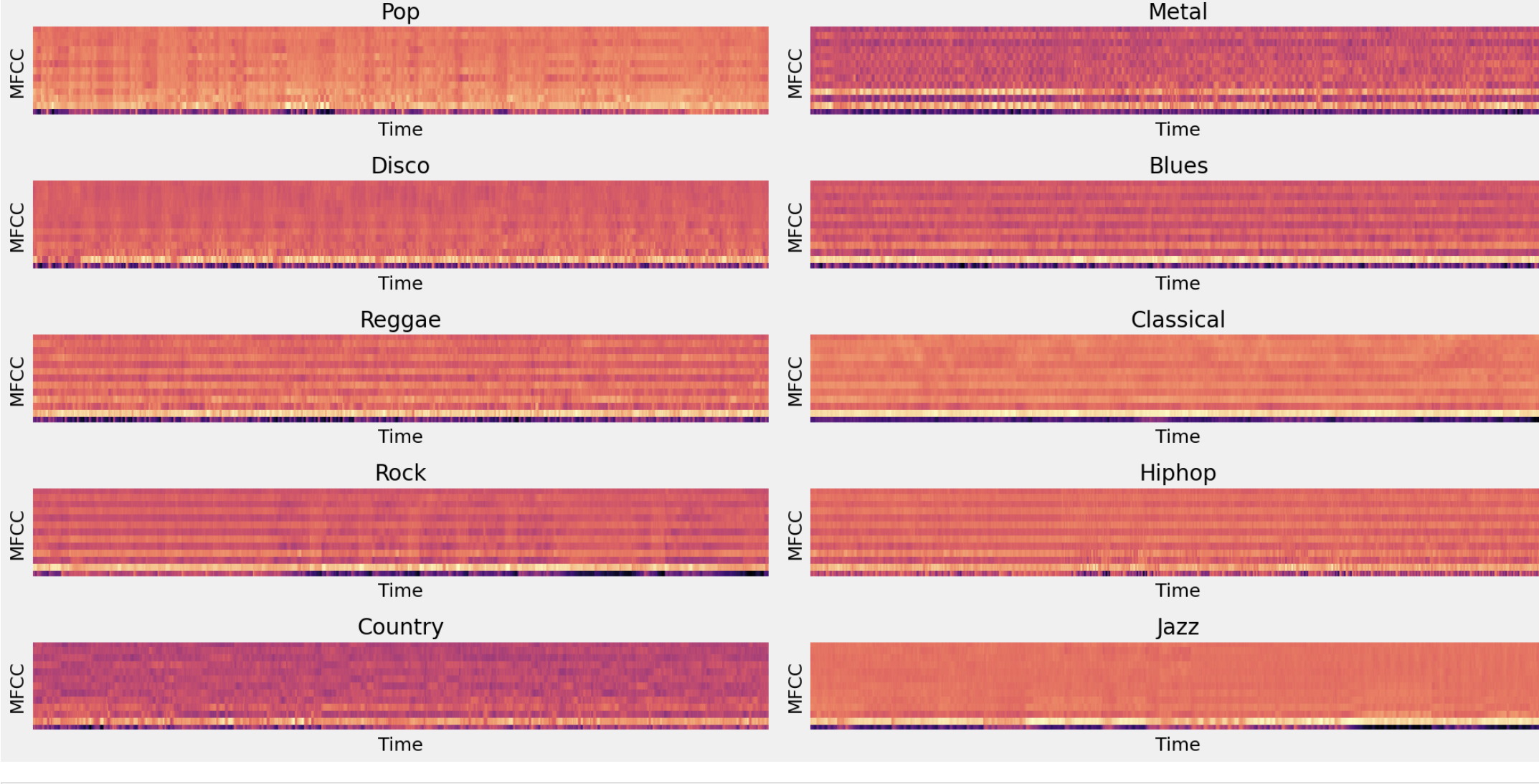
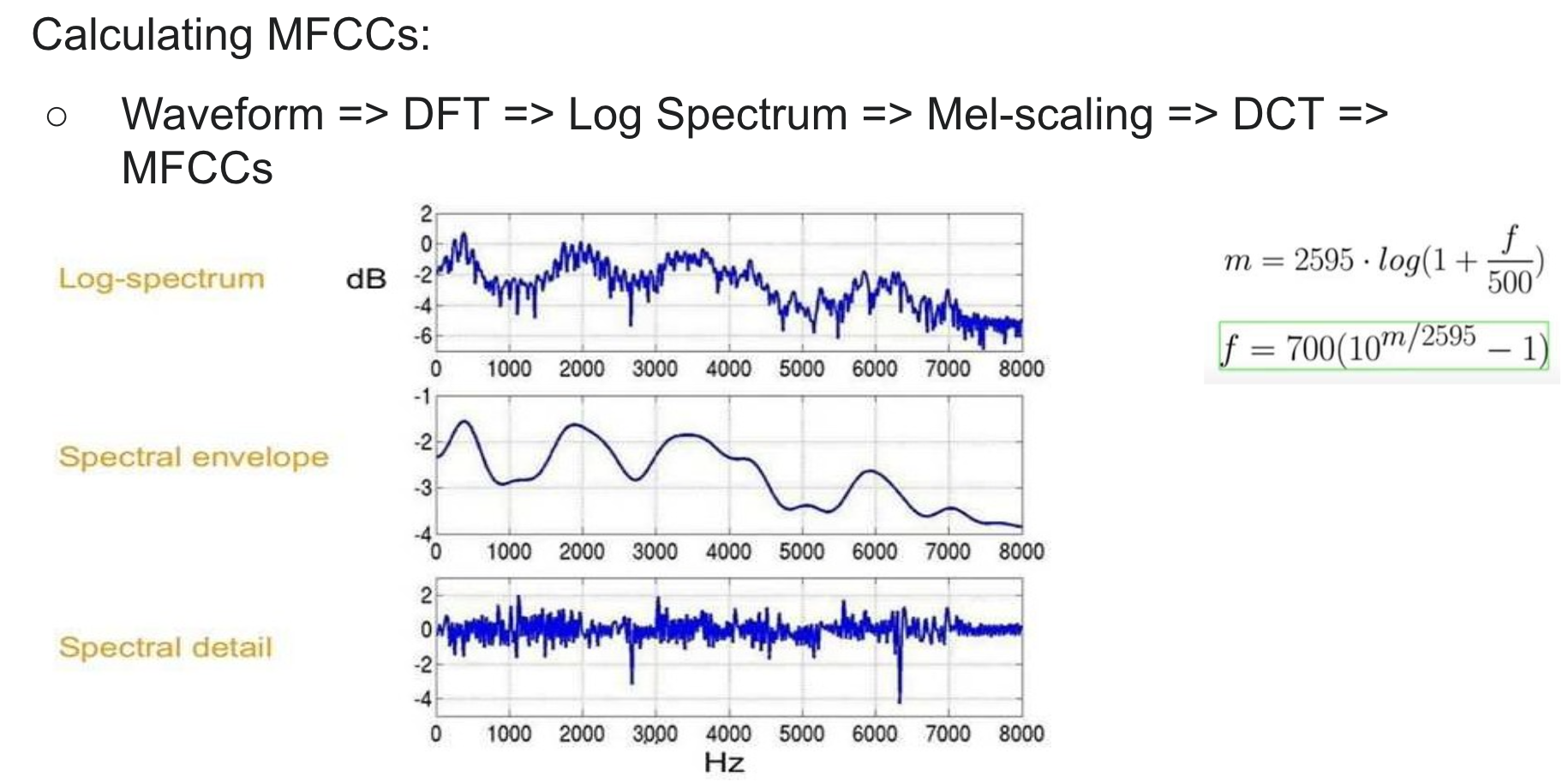
We needed a clear way to represent song waveforms for audio processing. We were introduced to MFCCs by existing music processing literature as a way to represent time domain waveforms as a small number of frequency domain coefficients. The Mel scale relates perceived frequency, or pitch, of a pure tone to its actual measured frequency. Humans are much better at discerning small changes in pitch at low frequencies than they are at high frequencies. Incorporating this scale makes our features match more closely what humans hear.

In sound processing, the Mel-Frequency Cepstrum (MFC) is a representation of the short-term power spectrum of a sound, based on a linear cosine transform of a log power spectrum on a nonlinear Mel scale. Mel-Frequency Cepstral Coefficients (MFCCs) are coefficients that collectively make up an MFC. MFCCs are extracted from all the audio files in the GTZAN dataset. Each audio file is of 30 seconds duration, which is further divided into 10 segments to derive the MFCCs. A JSON file is created to store the MFCCs of all the audios with their respective genres.

Artificial Neural Network (ANN)

Conceptual Overview

An Artificial Neural Network (ANN) is based on a collection of connected units or nodes called artificial neurons. Each connection transmits a signal to other neurons. An artificial neuron that receives a signal then processes it and can signal other neurons connected to it. The “signal” at a connection is a real number, and the output of each neuron is computed by some non-linear function of the sum of its inputs. The connections are called edges. Neurons and edges typically have a weight that is used for adjustments as learning proceeds. The weight increases or decreases the strength of the signal at a connection. Neurons may have a threshold such that a signal is sent only if the aggregate signal crosses that threshold. Typically, neurons are aggregated into layers. Different layers may perform different transformations on their inputs. Signals travel from the first layer (the input layer) to the last layer (the output layer), possibly after traversing the layers multiple times.

Implementation Details

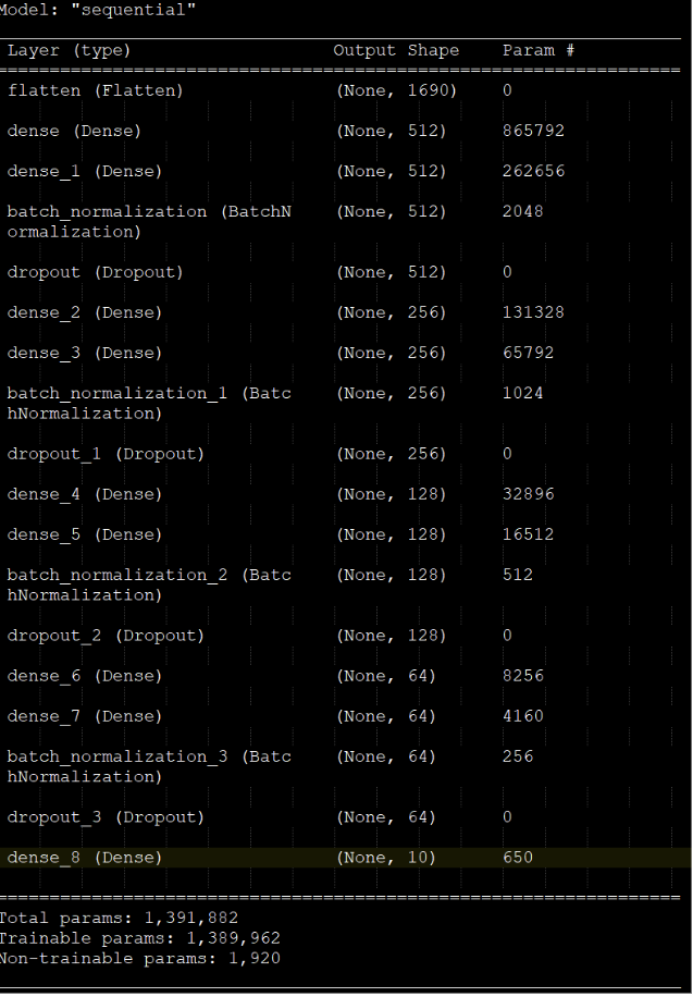
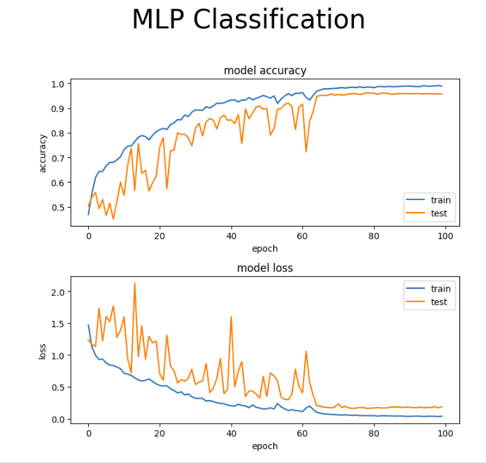
A 9 layer deep neural network, with dropout layers for regularization and batch normalization layers for stabilizing the learning process, was trained on the MFCCs extracted with a batch size of 24, for 100 epochs.
The Adam optimizer is used with a learning rate of 0.01 and cross-entropy loss is monitored along with accuracy as a metric.
The “rlprop” [ReduceLROnPlateau] callback has been setup as well, in order to reduce learning rate when a metric has stopped improving.
We have used GTZAN dataset [link : GTZAN Dataset - Music Genre Classification | Kaggle] for training. The GTZAN dataset is the most-used public dataset for evaluation in machine listening research for music genre recognition (MGR). The files were collected in 2000-2001 from a variety of sources including personal CDs, radio, microphone recordings, to represent a variety of recording conditions

Findings

Fig.3 - Graph of ANN

Fig.4 - Confusion Matrix

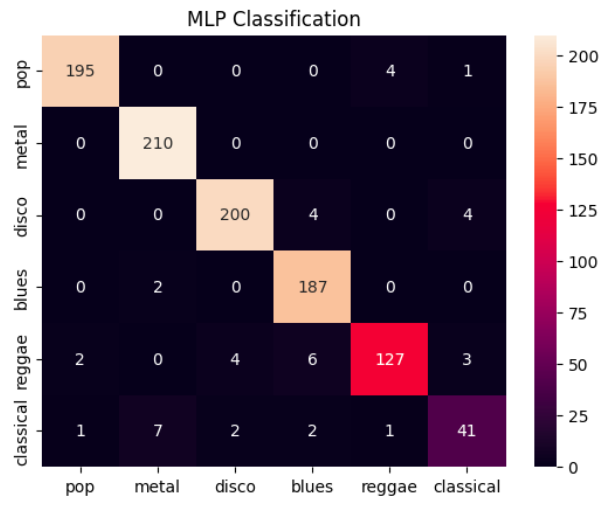
The matrix above tells us out of all cases for respective categories, how many cases have been correctly classified. For ex: For pop genre, 78 have been correctly classified. 6 cases for pop have been misclassified as disco, 2 have been misclassified for blues and so.

The training reached convergence after training ~1.4 millions parameters at around 35 epochs.

Long Short Term Memory (LSTM)

Conceptual Overview

Different from other Neural Network (NN) techniques, RNNs supply time-related context-based information to make decision relying on connections formed in cycle. The plain RNN structure could not handle long-term dependencies as the issues relating to vanishing gradient might arise. Therefore, Long-Short Term Memory (LSTM) was suggested as it can make another connection state present from successfully updated current activations. The LSTM is a branch of the RNN. RNN differs only slightly from conventional neural networks in terms of design. The stored historical data is used to make predictions about the future output. Additionally, LSTM is a brand-new, improved division that solves the issue of long-term dependencies. Even so, RNN makes use of the stored data to make predictions about the future based on the past. When there is a significant difference between the current situation and the situation from which the information must be drawn, the information cannot be linked.

Implementation Details

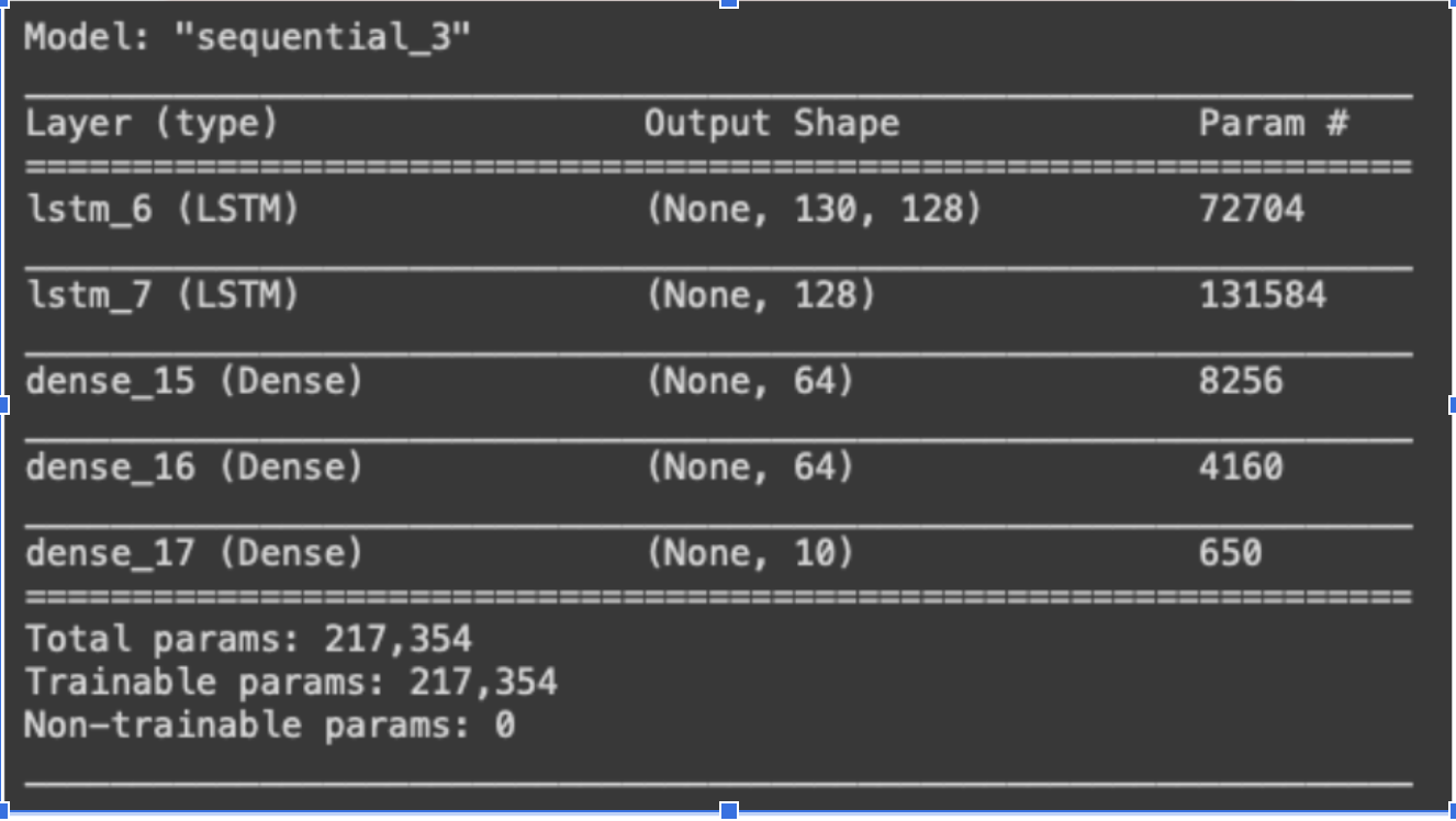
An LSTM network was built consisting of two LSTM layers and three fully connected dense layers.
Adam optimizer with a learning rate of 0.0001 was used.
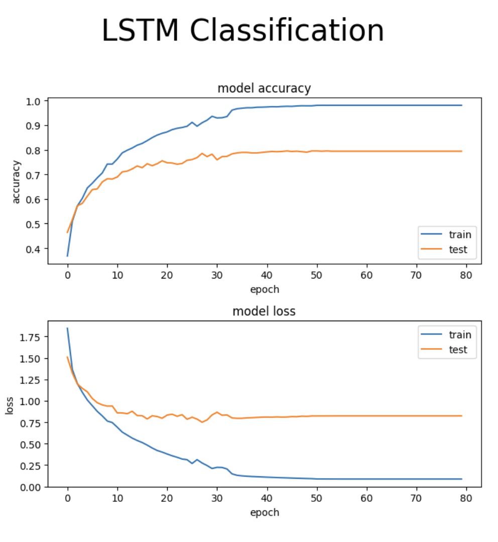
Cross-entropy loss and accuracy were set as the metrics and the network was trained for 80 epochs on data with batch size of 32.

Findings

Fig.3 - Graph of LSTM

Fig.4 - Confusion Matrix

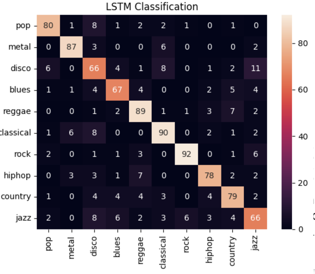
The matrix above tells us out of all cases for respective categories, how many cases have been correctly classified. For ex: For pop genre, 80 have been correctly classified. 6 cases for pop have been misclassified as disco, 2 have been misclassified as rock, 2 have been misclassified as jazz and so on.

The training reached convergence after training ~215k parameters at around 40 epochs

Convolutional Neural Network (CNN)

Conceptual Overview

A Convolutional Neural Network (ConvNet/CNN) is a Deep Learning algorithm that can take in an input image, weight the image's different features according to importance, and then distinguish between them. In the neural network, CNN uses convolution and pooling in alternating order.

Convolution: the network's use of kernels or grids (multidimensional weights) to apply to the input image. In our example, the kernel and spectrogram will be combined with a dot product, and the resulting grid will be passed to the following layer. CNN can use kernels as feature detectors because they can identify the type of MFFC's over a given period of time.

Pooling: shrinks the image and collects the kernel-identified features. The size of the feature maps is reduced by pooling layers. As a result, it lessens the quantity of network computation and the number of parameters that must be learned. An area of the feature map produced by a convolution layer is summarized by the pooling layer's features.

Implementation Details

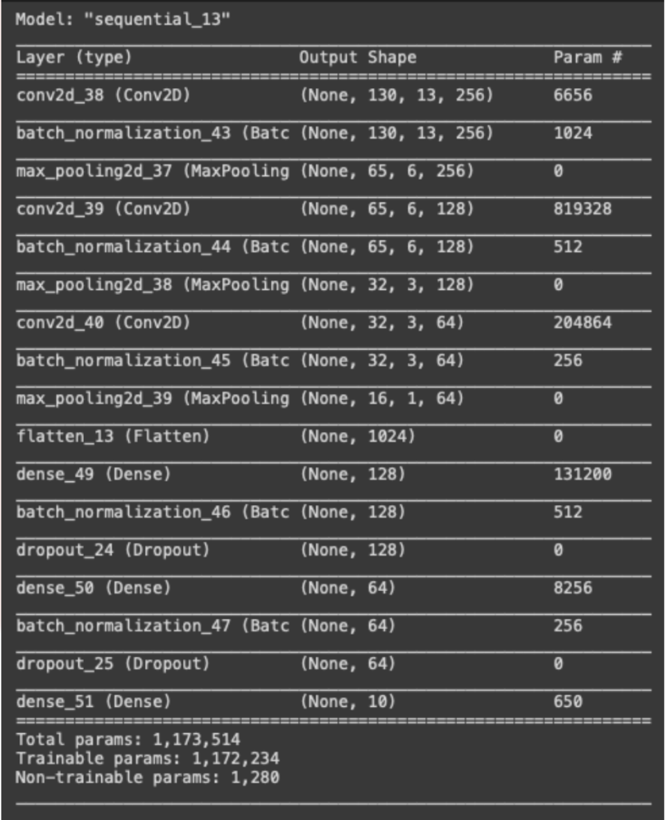
A ConvNet is constructed by using 2D convolutional layers, batch normalization layers, and max pooling layers for down sampling the feature maps.
The optimization algorithm used is Adam and the learning rate is set to 0.001.
Cross-entropy loss and accuracy are used as metrics and the network is trained for 80 epochs on data with batch size of 32.

Findings

Fig.3 - Graph of CNN

Fig.4 - Confusion Matrix

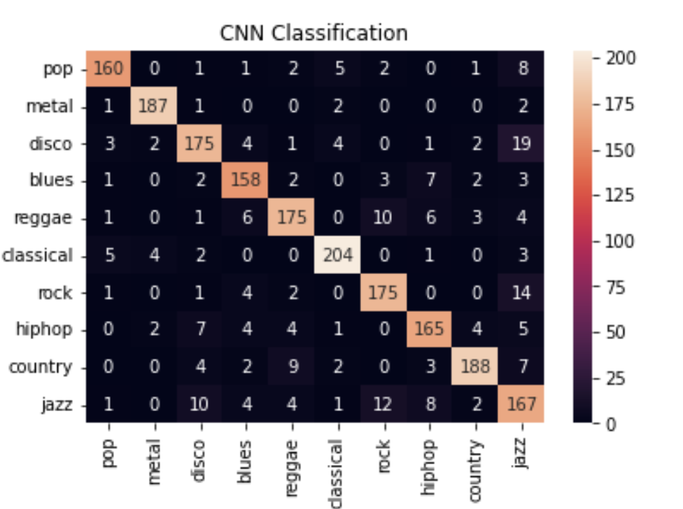
CNN:The matrix above tells us out of all cases for respective categories, how many cases have been correctly classified. For ex: For pop genre, 160 have been correctly classified. 6 cases for pop have been misclassified as disco, 5 have been misclassified as classical and so on.

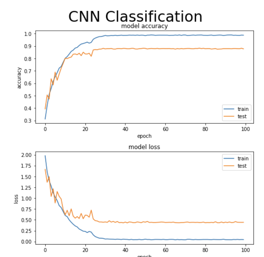
The training reached convergence after training ~1.2 million parameters at around 30 epochs

Conclusion

Following are the conclusions we made:

From the graph of CNN we can deduce that, CNN requires very few parameters to reach a answer as compared to dense layer models.
In CNN, the use of Kernel as filter hepls it to detects the feature of the image(spectrogram of MFCC) easily.
LSTM can understand the context more efficiently than other models because it is capable of predicting the next step based on previous data points.
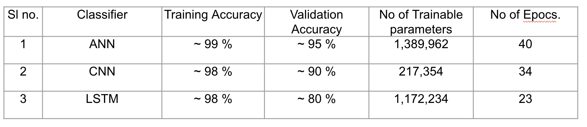
The final result of ANN, LSTM and CNN can be deduced from the following table. Accuracy of the deep layer network i.e ANN is best, because it is having the most layers. If we keep the number of layers constant in all the models, LSTM would have given the best results. We increased the number of layers in ANN on purpose, just to find out that how many layers would be required for a primitive method like ANNs to outcast the performance of LSTM. Out of all the 3 models, LSTM proves to be the best in terms of performance of the training as we got similar accuracy to CNN but the number of trainable parameters were significantly less and less number of epochs were required to reach convergence.

Future Work

We can use basic Machine learning Algorithms like KL divergence, Random Forest and KNN to classify music and compare them with the existing ones.
More interesting future work that can be done is eveloping a system for auto- matically creating a new compound by blending western music with classical music. The idea behind this work is motivated by various existing applications which make use of artificial intelligence for automatic music generation and remixing.

References

[1] Haggblade, M., Hong, Y., & Kao, K. (2011). Music Genre Classification.
[2] Hoang, L. (2018). Literature Review about Music Genre Classification.
[3] Agrawal, M., & Nandy, A. (2020). A Novel Multimodal Music Genre Classifier using Hierarchical Attention and Convolutional Neural Network.
[4] Mandel, M., & Ellis, D. (2006). Song-level features and svms for music classification. In In Proceedings of the 6th International Conference on Music Information Retrieval, ISMIR (Vol. 5).
[5] Bahuleyan H (2018) Music genre classification using machine learning techniques, Sound (cs.SD); Audio and speech processing (eess.AS)
Team Members
- Aayushi Gautam
- Visheshank Mishra