Hierarchical Time Series Forecasting on Walmart Products Unit Sales -- Milestone 2
Project Source and Links
Our Code and ImplementationMain paper: Hierarchical forecasting with a top-down alignment of independent level forecasts (arxiv.org)
Author's Github
Figure
Conceptual Review
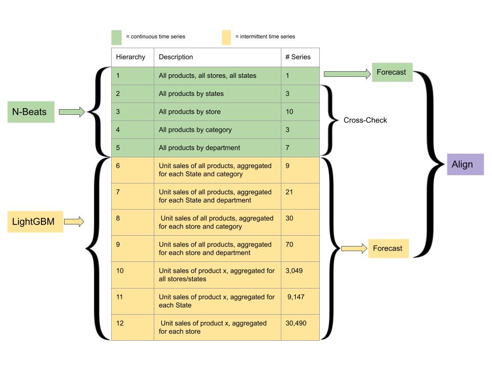
The main method this paper uses is combining two machine learning algorithms, N-BEATS and LightGBM, for different tasks within the hierarchical-forecasting-with-alignment framework. N-BEATS uses a deep stack of full-connected layers: 30 stacks of depth 5 and a total depth of 150 layers. It's composed of two residual branches to form a doubly residual stacking architecture: one runs over the backcast prediction of each layer, the other the forecast branch of each layer. This allows it to run without a massive data source or utilizing extensive feature engineering. The authors use the GluonTS implementation of N-BEATS rather than the original, as it requires less hyperparameter tuning of the variable representing the historical range of length for each selected time series. GluonTS instead reduces computational requirements by randomly selecting a time series and a starting point within it. This paper trains N-BEATS using the top five levels data. LightGBM uses gradient boosting decision trees: it first uses the decision tree algorithm to partition inputs into tree structures. Since the decision strategy for trees is so weak, it uses gradient boosting algorithms to aggregate predictions and improve performance, making the ultimate prediction based on the tree. This is used for the bottom level to model the intermittent time series.
Implementation Details
The data we used is found at the Kaggle competition this paper was a submission for. It consists of five csv files, whose summaries are courtesy of the Kaggle page:
- calendar.csv - Contains information about the dates on which the products are sold.
- sales_train_validation.csv - Contains the historical daily unit sales data per product and store [d_1 - d_1913]
- sample_submission.csv - The correct format for submissions. Reference the Evaluation tab for more info.
- sell_prices.csv - Contains information about the price of the products sold per store and date.
- sales_train_evaluation.csv - Includes sales [d_1 - d_1941] (labels used for the Public leaderboard)
We took this data and ran it through the model as found on the author's Github. The author's code consists of four Python Notebooks and a dataset. The author's description of these is as follows:
- m5-simple-fe-evaluation.ipynb: feature preprocessing notebook
- m5-final-XX.ipynb: bottom level (lvl12) train and predict notebook
- m5-nbeats-toplvl.ipynb: top level (lvl1-5) train and predict notebook
- m5-alignandsubmit.ipynb: notebook to align bottom level with top level results
- gluonts-20200710T072218Z-001.zip: modified glutonts version (added lookahead to Trainer)
We followed the author's README instructions. This involved first running m5-simple-fe-evaluation.ipynb for feature preprocessing. We then trained the bottom-level model using m5-final-XX.ipynb five times, using five different loss multipliers as recommended by the authors. We used the five bottom-level model results when training the top-level model using m5-nbeats-toplvl.ipynb. We did this three times for each of the changes to our hyperparameter we tested, batch number. Finally, we aligned the results with m5-alignandsubmit.ipynb, which gave us the errors and visualizations. For all hyperparameters other than batch number, we used the suggested values from the paper.
Findings
Our goal for this milestone was to figure out how to successfully run the author's code to generate predictions based on time-series data, using their hierarchical-forecasting-with-alignment approach, while also analyzing their code for potential opportunities to test hyperparameters. We also aimed to test variations in performance on one hyperparameter.
For this first task, running the author's code, we ran into a few difficulties. The first was that this ended up being a very computationally expensive process to run. We were unable to run it on the base version of Google Co-lab, so one member of our group purchased Colab Pro+, while the other tried running the code on the Discovery cluster. We were unable to figure out how to install dependencies on the cluster, so we switched the other method of running to using the clusters on Kaggle. For the majority of our computation, however, we used the cluster on Colab Pro+, which allowed us enough compute resources to run their code with different hyperparameters. Getting the code to run was fairly straightforward once compute resources were no longer a problem, as the authors did a good job documenting their code and the points at which we needed to update for our own environment. However, even with sufficient compute resources, it took many hours for their code to run. While this meant we were grateful to have started early and had enough time for the code to run so that our experiments could be conducted, with the short turnaround for Milestone 2 it also meant that, to have enough time to complete our analysis, we could test fewer hyperparameter adjustments than we had hoped. Since for each hyperparameter change we needed to run the entire top-level N-BEATS model again, we could change fewer parameters.
Another difficulty we ran into was setting up GPU support for the top-level model. Due to this model being a few years old, there were some conflicts with the dependencies for cuda on CoLab being out of date from what the model was using. We needed to figure out how to install the correct version of mxnet. We were unable to fix this on the desktop and used CPU for the majority of our calculations. We intend to look into this further for the final project.
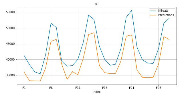
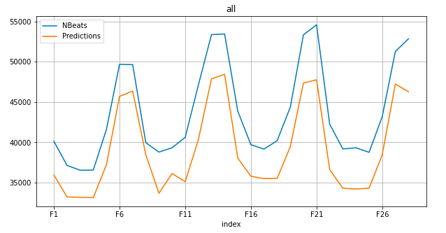
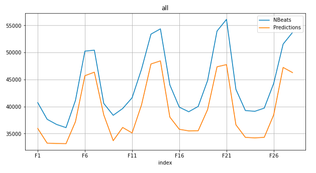
The results for our experiments and supporting visualizations are given below. We note that all errors and graphs are the aggregate values, instead of dividing it by state, store, and product category as the paper does. This was done to conserve space and focus on the aggregate data. We note that the error is lowest for the lowest number of batches per epoch, with a root mean squared scaled error of 0.66561. We found a significantly higher error than reported in the paper. The paper's error values for an epoch of 10 and number of batches per epoch at 1000 for all categories was 8.2742 x 10⁻⁵, compared to our value of 0.858572. This ran counter to our expectations, as we believed we were running the code identically to what the authors performed. We do not know why this is, and intend to investigate this further in the final project.
Experiments:
- Number of batches per epoch: 100
- start time: 1665460744.130973 - Monday, October 10, 2022 11:59:04.130 PM
- end time: 1665462137.675431 - Tuesday, October 11, 2022 12:22:17.675 AM
- total runtime: 0.38 hours
- rmsse: 0.66561
- mean_error: -4562.591561
- mean_abs_error: 4562.591561
- rmse: 4826.258199
- Number of batches per epoch: 500
- start time: 1665435559.5475013 - Monday, October 10, 2022 4:59:19.547 PM
- end time: 1665442691.4661298 - Monday, October 10, 2022 6:58:11.466 PM
- total time: 1.98 hours
- rmsse: 0.793228
- mean_error: -4651.500601
- mean_abs_error: 4651.500601
- rmse: 4800.218426
- Number of batches per epoch: 1000 (paper's recommended value)
- start time: 1665444252.39971 - Monday, October 10, 2022 7:24:12.399 PM
- end time: 1665458178.277721 - Monday, October 10, 2022 11:16:18.277 PM
- total time: 3.8683333 hours
- rmsse: 0.858572
- mean_error: -5031.394016
- mean_abs_error: 5031.394016
- rmse: 5217.090655
Next Steps
This beginning implementation was highly valuable in informing our project's scope and we ironed out a number of difficulties early-on that will allow us to focus on analysis and processing moving forward.
Since the size of data used the paper is large, we have to spend so much time to train the models, which makes us hard to try out different factors, such as learning rate, that might influence the accuracy. Therefore, we are going to use a reasonable size of time series dataset from GluonTS, which is a python package for deep learning time series models.
We are going to use the 'm4-monthly' dataset, It is part of the dataset that is being used in the fourth edition of the Makridakis forecasting Competition. In addition, the model used in the paper is too complicated to make readers have a clear understanding on how the deep learning model trains time series data. We are going to focus on making an explicit and detailed tutorial about the concepts behind the code of GluonTS.
The content of our explanation of GluonTS will include the architecture of the models, the techniques of model training, and so on. Therefore, people who read the paper can generate better understanding of the code used in the paper and the concepts behind time series data and deep learning.
References
[1] Anderer, Matthias and Li, Feng (2021). Hierarchical forecasting with a top-down alignment of independent level forecasts. arxiv.org.
Team Members
Levi Kaplan, Ming Luo