CS 7150 Final Project
Deep Learning by Professor David Bau, Fall 2022
Probing Latent Diffusion
Andrew Lemke & Lakshyana KC
Introduction
Diffusion models’ high quality generations and capability to condition on text brought praise and interest to this development. Examination of the model’s denoising process leads one to the traditional visualization, which shows each intermittent latent processed through the VAE, producing a series of images showing a form appearing out of noise. This interrogation leaves many questions about the models behavior, especially as much of the first half of this visualization is too noisy to determine what actions the model is taking. The nature of the prompt’s grammar and impact is also unclear. We aim to answer these questions by probing the latent space of the model, and visualizing the results.
To discover more about the diffusion process, we constructed four probes that reveal behavior of the model not observable in the traditional visualization. Probes 1 and 3 indicate the model takes only a few steps to determine the sketch of the final output, with probe 3 showing the model’s focus at various steps. Probe 2 investigates the impact of conditioning between generations with good and bad prompt synthesis.
Probe 4 performs a text-image attribution analysis on the Stable Diffusion model with the help of the diffusion attentive attribution maps (DAAM) method, which is based on interpreting the model using aggregated and upsampled cross attention scores [6]. We use this method to probe into the stable diffusion model’s visual reasoning abilities such as compositional reasoning, object recognition and counting, and spatial and object-attribute relationship understanding. This investigation indicates that the model demonstrates a higher accuracy in representing the correct actions and objects based on the prompts in the generated image, compared to their counts and relationships. In addition, when evaluating the model’s general performance after categorizing the attention scores for a word by its parts of speech, certain word types such as nouns and verbs were observed to have a higher attention score distribution over the generated images in comparison to adjectives and numerals.
While comparing the model’s outputs for the same prompt over multiple experiments, the model showed varying performance in several prompts. While some experiments showcased an accurate heat-map and image generation that captured each object and relationships conveyed by the prompt, others had some attributes or objects from the prompt missing in several cases, indicating a relatively weaker visual reasoning skills of the model in comparison to what its realistic image generation capabilities might indicate.
Background
Diffusion Models
Diffusion models are generative models that learn to gradually remove noise from data. In inference mode, they generate data after iterative denoising a random initial seed. These models gained popularity in the image generation space where they can be trained to generate images conditioned on a text input, which is the kind of model we explored here.
The idea for this type of model started in 2015 with Sohl-Dickstein et al., and was improved upon in 2019 and 2020, where it gained enough capability and traction to break out on to the image generation scene (2).
The following model is often presented to describe the noising process. An image starts at time t=0, and q gradually adds noise to the image over a number of steps until the image is pure gaussian noise at t=T. The reverse process p removes the noise at a particular step. (1)
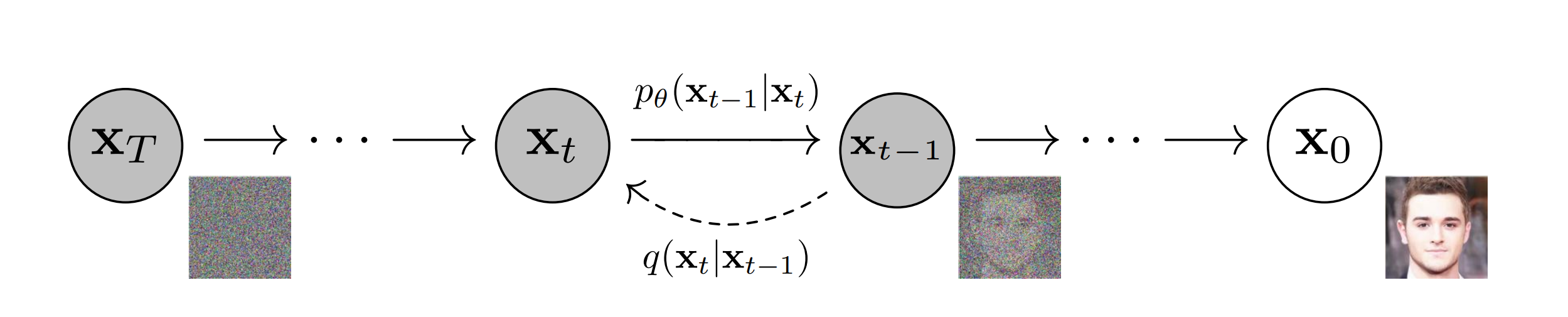
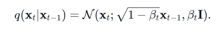
Writing the q process is fairly simple. To calculate the q at the next timestep, we sample some gaussian from the previous timestep with a mean and variance that also depend on some parameter beta . Beta increases with t between (non inclusive) 0 and 1. The schedule of the betas can be altered as a hyperparameter of the process. The key point is that at time t=T, the image must be noised so much that it is indistinguishable from gaussian noise, in other words, no “signal” remains.
The p process is the hard part, in fact, it is intractable as it requires knowing the total distribution of all images. The diffusion network is trained to learn how to do the p process. In practice, Ho et al. finds predicting the noise added “performs approximately as well as predicting [the mean] when trained on the variational bound with fixed variances, but much better [performance] when trained with our simplified objective,” alluding to some theoretical simplifications made in their paper.
In architecture, the noise predictor relies on U-nets. The timestep is incorporated as a positional embedding. The HuggingFace implementation (whose weights are freely available) (3) is based on the Ho et al. implementation, who adapted Wide ResNets from Sergey Zagoruyko and Nikos Komodakis (4) with minimal changes.
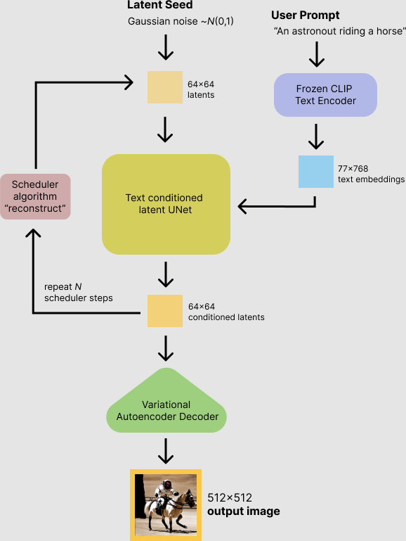
The text to image model investigated in this report relies on a diffusion model, as described above, in combination with a text encoder to embed the prompt, and a VAE to transform the latent produced by the diffusion into image space. Training data comes from a set of images and associated texts.
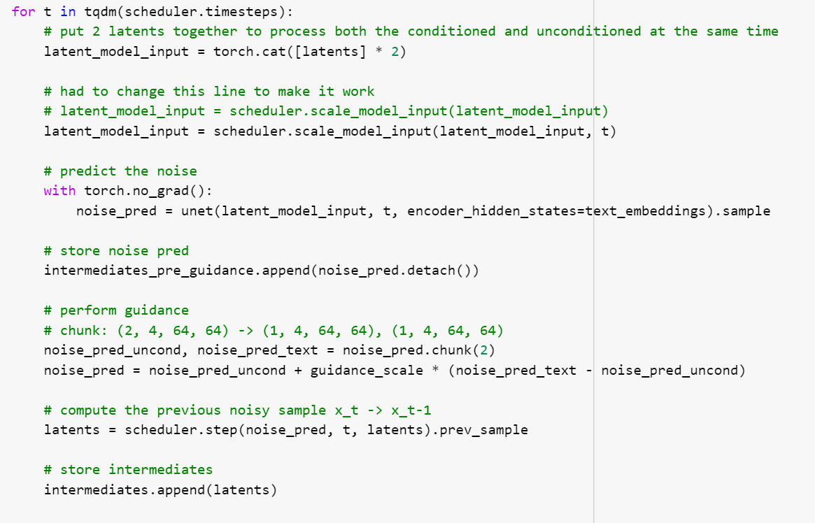
In code, the process is slightly more complicated. To increase performance, the impact of the conditioning is boosted by a factor called the guidance scale. When the diffusion loop runs once, it actually diffuses two latents. One latent is diffused with the prompt and another is diffused without it, which in practice happens by conditioning it on an empty string embedded by the text encoder. The difference between these two can be seen as the impact of conditioning. It is calculated by subtracting the unconditioned latent (empty string one) from the conditioned latent (prompt one). This difference is multiplied by a scalar in the neighborhood of 5-10 and added to the unconditioned latent, increasing the impact of the prompt during the diffusion process. The code below is based on the “writing your own diffusion pipeline” section of citation number 5.
Diffusion Model Attribution
With increasingly complex neural network models in use, attribution has become an important method to better understand the basis of a model’s predictions. Attribution is a way to characterize a model’s response by identifying the parts of an input that are responsible for its output [7]. Most of the attribution methods currently in use are mainly perturbation and gradient based [8,9]. The gradient based methods involve some modification of the backpropagation algorithm to backtrack the network activations from the output back to the input, which when applied to vision models, result in saliency maps highlighting important regions in the input image [9]. The perturbation methods perform analysis of the effects of perturbing the network’s input on the corresponding outputs by observing the effects of selectively removing or occluding parts of the input on the output [9, 10].
Although the gradient-based attribution is used for visualizing the saliency maps for vision models, it is not feasible for diffusion models, as the costly backprogation computation is needed for each pixel across all the timesteps and the perturbation attribution are challenging to interpret owing to high sensitivity of diffusion models to even minor perturbations [6]. As a result, Tang et. al. have proposed a text-image cross attention attribution method called diffusion attentive attribution maps (DAAM) to visualize the influence of each input word on the generated image output. Their method enables a pixel level attribution map generation for each word of the prompt. To obtain the maps, this method upscales the multiscale word-pixel cross-attention scores obtained for the latent image representations in the denoising sub-network, and aggregates these scores across the spatio-temporal dimensions to then overlay each map obtained for an input word over the generated image [6].
We thereby apply the DAAM attribution method to probe into the stable diffusion model to visualize the spatial locality of attribution conditioned on each input word. This attribution technique also enables a way to qualitatively study the stable diffusion model’s understanding of concepts and behavior for input words based on their parts of speech.
Acknowledgements
The code for probe 1 is derived from the first homework of this class. The code for probe 2 and 3 comes from the “writing your own diffusion pipeline” section of the HuggingFace blog post “Stable Diffusion with Diffusers” (see citation 5). Both of which use the model architecture and weights from HuggingFace’s “Stable Diffusion v1.4,” which is citation 3. Without these weights none of this analysis would have been possible. Probe 4 experiment is uses pretrained model weights from HuggingFace’s “Stable Diffusion v1.4” and “RunwayML v1.5” models, and applies the code open-sourced by the authors of the DAAM paper [6] to implement further analysis and experiments. In addition, the words used for generating the prompts are sourced from the top 1000 frequently occurring words in the COCO caption data [10].
Probe 1: “Rip Out” Images from Intermediate Latents
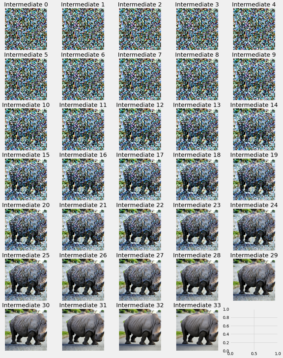
The standard visualization for latent diffusion takes the intermediate latents at various steps through the diffusion process. These intermediates then pass through a VAE to transform from latent space to image space. The effect does convey the principle idea behind diffusion–showing an image emerging from noise–but presents frustration. In a diffusion of 100 steps, the first 20 or so will just appear to be noise.Rapidly and without warning, an image appears. The primary subject (as indicated in the prompt) and background details both become distinguishable. We do not have insight into how the model came to this decision, whether the generation ever altered from its initial notion of the image, or see where focus is on each step. Questions arise like “what happens in the first 5 steps? Does the model randomly pick directions to push the image until one appears patterned enough to provide the diffuser with enough of an image to move forward with noise reduction?” and “Does the model change its mind?”
Methodology & Experiment
I continued the idea explained in the proposal–that I would try to get the model to “finish fast.” This can be done in 2 ways. The first is to alter the scheduling mid run to a schedule that informs the model to quickly finish the diffusion. For example, at step 30 of 100, change the schedule to have only 5 drastic steps to present the final image. The second method is to save a target intermediate from a diffusion run. The latent is then processed through a separate diffusion with the target schedule by using that latent as the starting seed of the diffusion. I elected to do the latter of the two.
The new effective schedule concatenates the original schedule of the latent until it gets to the target intermediate step and the new schedule in the second run. The below charts show the schedule for various targets and the cumulative sums of the schedules. The top of the peak in “quick finish 10” is the start of the new schedule.
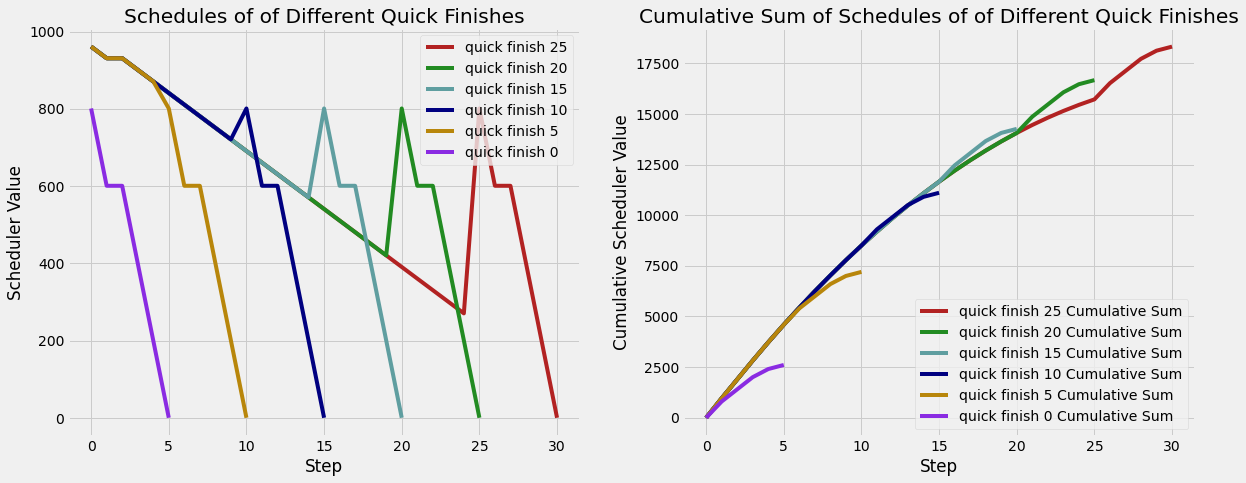
In practice, every intermediate latent was captured then passed though the quick finish diffusion, which was 5 steps. The number of steps to force the quick finish is a tunable parameter in generating these results. The guidance schedule in the second diffusion is also critical. The guidance scale is the factor to multiply the difference between the unconditioned (no prompt, just denoise) and the conditioned (denoise with prompt as input) latenets. A guidance scale of 0.0 means the generation uses no information from the prompt and simply removes noise. A scale of 1.0 means the diffuser works on the conditioned prompt. Scales above 1.0 increase the differences between the unconditioned and conditioned prompt, which is added to the unconditioned prompt, resulting in a larger prompt impact. We examined the results with a scale of 0.0 and 1.0.
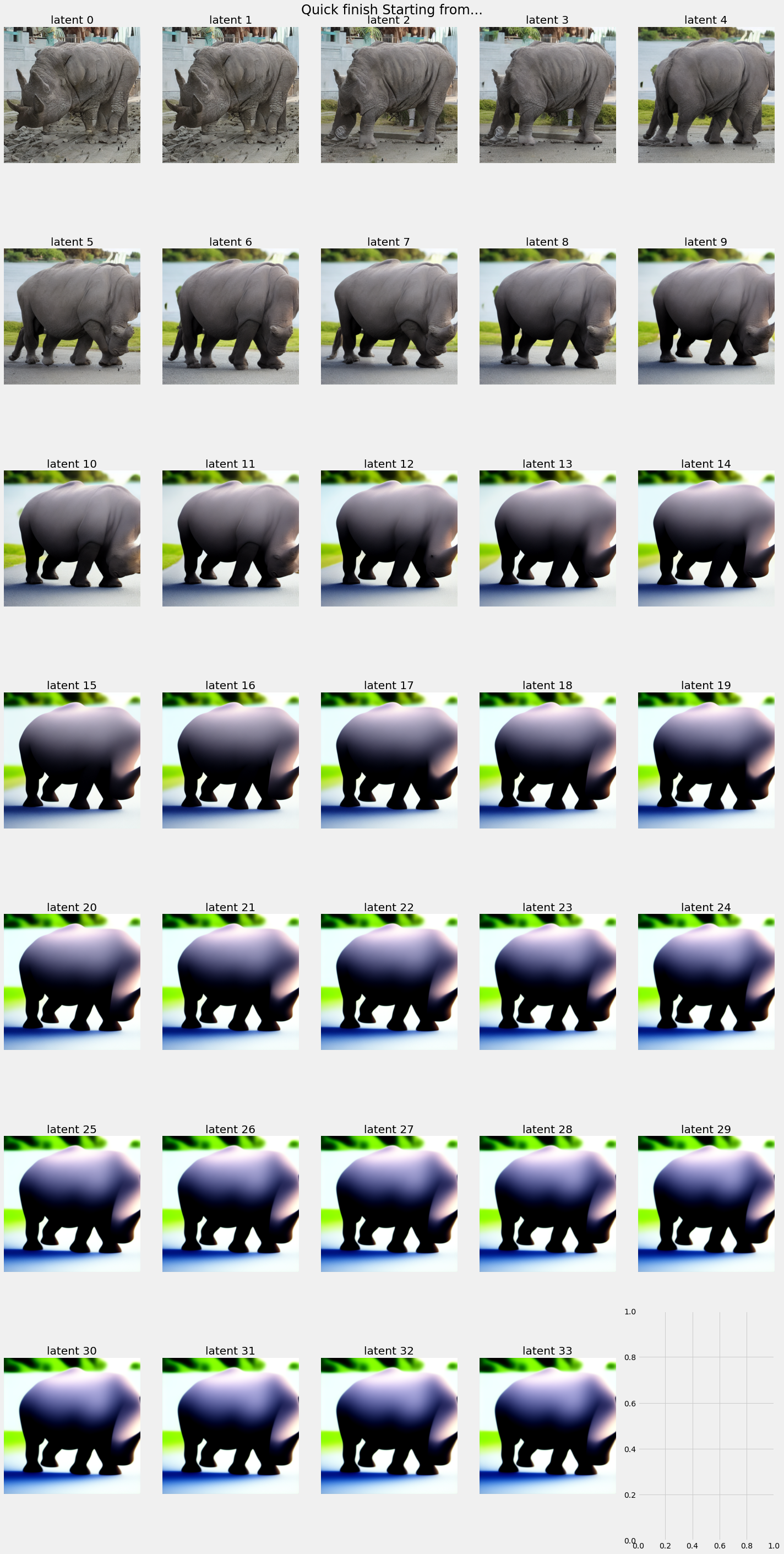
With 33 diffusion steps, we have 32 intermittent latents and the final latent which generates the output. We ran the quick finish diffusion of 5 steps on each of these latents to “rip out” the idea that may be contained in the noise. We focused our attention on the earlier latents, which appear as just noise if passed through the VAE before the quick finish. Our process generates an equal number of quick finish results (so 33). We ran the quick finish for a guidance of 0.0 and 1.0 though a 5 step quick finish diffusion.
Results
If the quick finish uses a guidance of 0, then there is no conditioning from the prompt, meaning the vector representation of “Rhino in a street” never influences the second diffusion. If the idea in this prompt is not present in the results until the 10th latent, then we can conclude the latents before that have not made appreciable progress toward the end goal of that image. Its appearance in the guidance scale of 0.0 run shows us when the idea appears in the intermediate latents by removing the noise that permeates the early latents without adding any information. Since no prompt information is included in the second diffusion, we can be sure that the model is simply removing noise from the latent from the first diffusion.
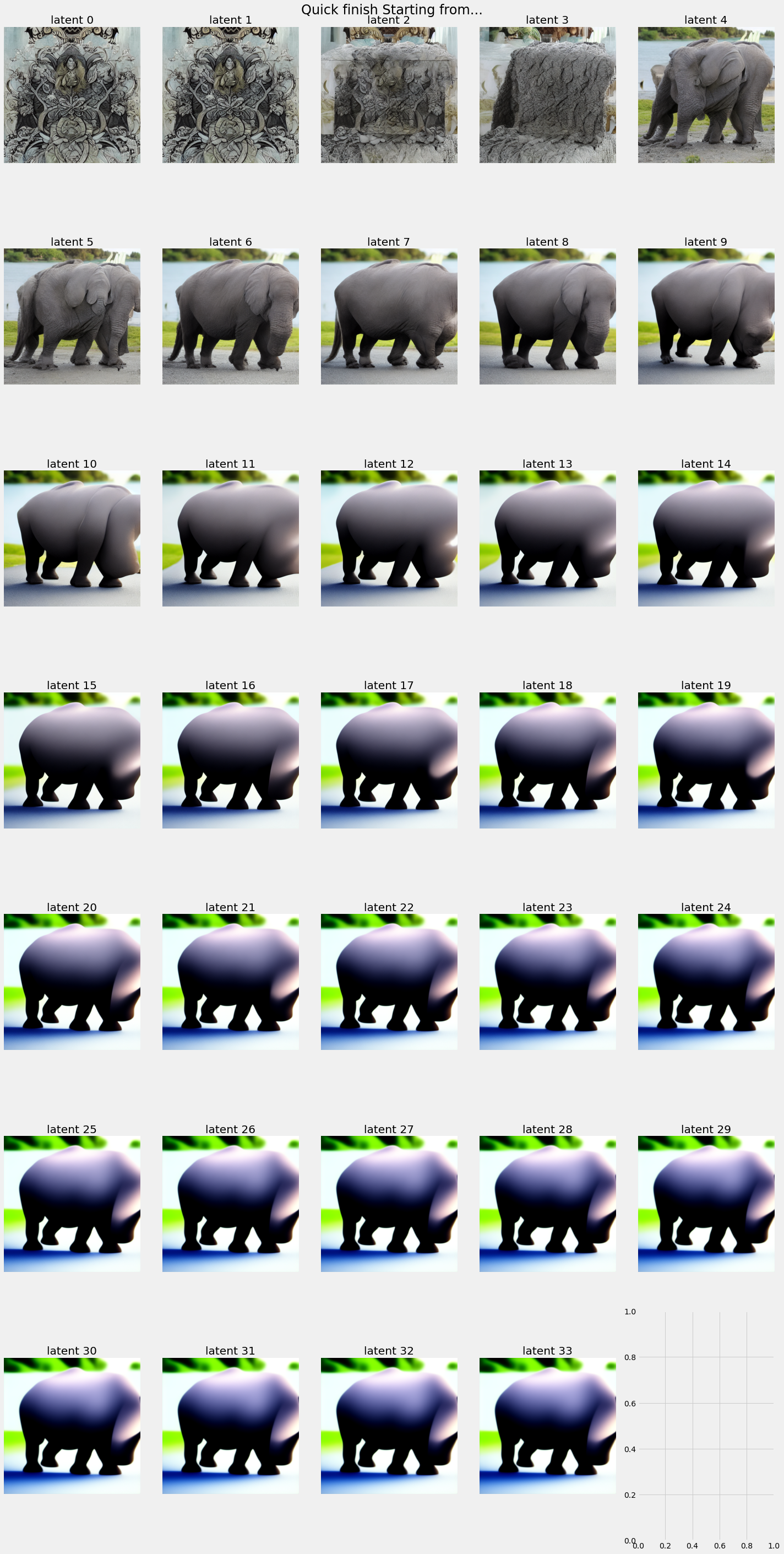
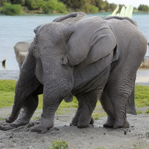
We can see from the first latent’s quick finish that the model has put 0 concepts from the prompt into the latent at this point. It appears abstract and vaguely monocolored.
The fourth image appears to have some sort of animal form in it, which morphs into the Rhino in later latents. Since the transition from this animal amalgamation to an actual rhino form is gradual, we are hesitant to pinpoint a specific step where the idea of a rhino appears in the latent. At step 4, we see an animal form, and by step 9, it appears like a rhino.
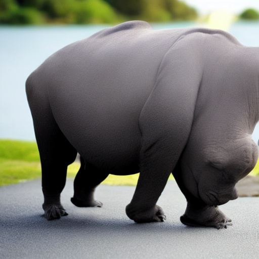
The concept of a street also comes about in the same range. The background still appears to be wild, as some jungle or outdoors area, but the foreground is pavement.
We observe an interesting effect when a late state latent passes through a diffusion model again as the seed. It comes out looking less detailed and more abstract. We think the model is simply not trained to perform under these conditions and its puzzling behavior is just a coincidence of this unusual situation. The model expects a very noisy image for most of the quick finish, so if a clean image is presented, the model acts unpredictably.
Over the course of many runs, we can profile the model. With the unconditioned (guidance scale 0.0) quick finish strategy, we will record the step where the prompt manifests in a discernible way. A value of 3 for this score means that latent has passed through 3 diffusion steps as it normally would before the quick finish. While “manifesting” is by nature subjective, we will specify that it is when one major physical object from the prompt appears in the diffusion. The average of 10 runs across different prompts and seeds is 12.3 steps. The total process is 33 steps.
When a guidance scale of 1.0 is used, we see the rhino from the first latent. A guidance scale of 1.0 is equivalent to diffusing with the prompt alone. This observation matches the results from the 0.0 guidance scaling run. The latent after run 0 in which guidance scaling of 1.0 has been diffused once with the prompt in the original run and 5 additional times in the quick finish with conditioning, giving it 6 total diffusion steps exposed to the prompt. In the 0.0 guidance scaling case, the 6th latent has been exposed to the prompt 6 times in the original run and 0 times in the quick finish. The rhino is visible in the image from the 6th latent.
Discussion
In the traditional visualization, the form of the prompt is not visible until about 40-50% of the way through the diffusion. Seeing the rhino appear earlier in the quick finish without conditioning tells us that the model is performing useful actions that move it towards a clean coherent image earlier than one would assume when using the traditional visualization. The interesting effect where the quick finish degrades quality in later runs motivated us to seek alternate visualizations or metrics that inform us of the model’s actions and progress throughout the diffusion process. The second attempt to answer this question is in probe 3
Probe 2: Conditioned-unconditioned difference patterns in results with good and bad prompt manifestation
Occasionally, the Huggingface model fails to produce the desired result, which happens when the text in the prompt is not matched or the resulting image possesses incoherence. In the first case, where the prompt is not followed properly, the impact of the guidance may not be strong enough. Alternatively, if the conditioning’s impact in the first part of the diffusion is not great enough, then the ideas in the latent may be “set” incorrectly or not enough. We investigate to see which, if any, is the case.
Methodology
To investigate the idea synthesis, we examined the magnitude of the difference between the conditioned and unconditioned prompts. Three methods were devised to calculate this difference. The first method is the simplest, it is the L2 norm of the difference between the conditioned and unconditioned latent. The latents are of shape (4, 64, 64) and the difference is too. The L2 norm is computed of this flattened difference. The second method looked to smooth out any differences due to changes in where objects borders are. If the conditioning translated an object left a pixel, a large difference would appear very great under the first method since there would be many many mismatches between the object and its shifted position after conditioning even though the only change is a translation one pixel leftward. To remedy this, the second method uses a 3d average pooling kernel of shape (4, 2, 2). 4 is the channel dimension, and (2, 2) are the spatial dimensions. After the pooling, the L2 norm of the difference of the conditioned and unconditioned latent is measured. The last method keeps the channels independent in pooling, using a (2, 2) average pooling kernel for each layer. Again, the L2 norm of the difference of the conditioned and unconditioned latent is captured. There is no padding in the second and third method, and each kernel’s stride length is set to 2, its spatial dimension.
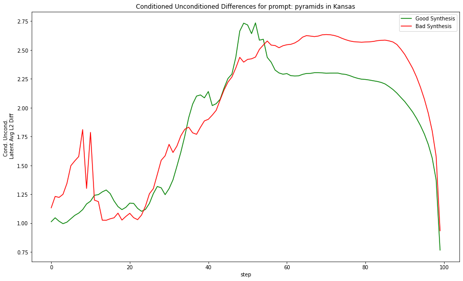
The idea for this investigation came when examining some series of runs for a single prompt. A pattern emerged when plotting the difference between the conditioned and unconditioned split by good or bad prompt synthesis (putting each thing specified in the prompt into the image). The runs with good prompt synthesis have conditioning that rises and peaks mid way through before abating and then dropping off. The poorly synthesized images have a conditioning difference that rises and plateaus until the end. The below figure shows this effect using the third strategy pools at each layer.
Experiment
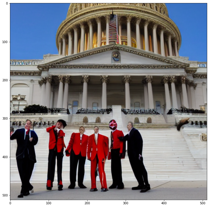
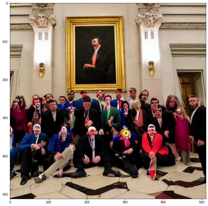
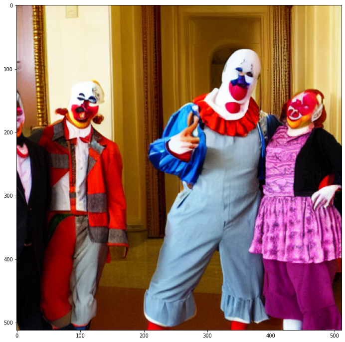
To examine the pattern, many instances over many prompts must be run, and the results must be classified as good or bad. A third classification of neither is used for images that are somewhere in between. The below example shows one of our classifications for the prompt “Clowns in the US Capitol Building.” A good synthesis of ideas does not always indicate a high quality result; an image may include the whole prompt but look distorted.
The actual effect of the three different methods of difference calculation is slight. We prefer the last way since it provides the benefit of pooling over minor translation issues but keeps the channels separate, since there is no reason to pool over them since each channel may be different and not related in value to the other channels in a way that makes pooling over channels interesting or useful. An example for an image points this out. Suppose image A is all red and image B is all blue. The difference between these images is drastic. A-B will be 255 in all the red channels, -255 in all the blue channels and 0 in the green channels. A 3d 1x1 average pooling strategy will perform (255 + (-255) + 0) / 3 = 0, negating the clear color difference.
A total of 130 images were generated, a prompt was run for 20 or 30 times, with varying seeds. Analysis seeks to capture the trend in the Kansas plot using a variety of mathematical strategies. The metrics are: the location of the maximum difference, the sum of the differences both pre and post the maximum index, the ratio of those two numbers calculated on a per diffusion basis, the pre and post run slope over the 10 preceding or trailing steps, and the mean difference for steps 60 to 80 and for steps 18 to 24. These statistics were run for the raw differences and for the differences scaled so the maximum is 1.0.
Results
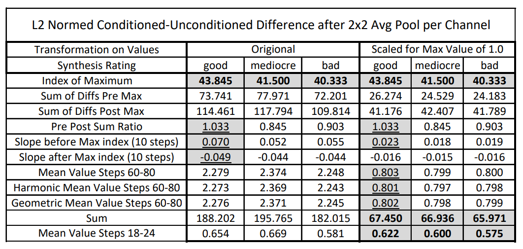
The results prove that over many different prompts and seeds, the pattern observed in the several runs of the “pyramids in Kansas” prompt does not hold true to a great extent. Only in the index of the maximum difference, the scaled sum of all differences for all steps, and the mean of the scaled sum for steps 18-24 followed a trend where the good and bad synthesis values are on opposite extremes and the mediocre synthesis is somewhere in between. I would expect more metrics from above to follow this trend if the trend was significant.
The below plot shows the first method, the L2 norm of the difference, and the third method, the L2 norm of the difference between the conditioned and unconditioned latents after a 2x2 average pooling applied to each layer independently. The plots for both method 1 in the solid lines and method 3 in the dashed lines are shown below.
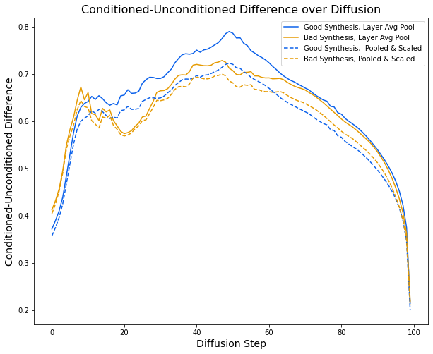
We observe a pattern here different from the “pyramids in Kansas” run. The pattern is still distinct enough to be present in this plot where 58 good runs and 36 bad runs were averaged to produce the lines. The poorly synthesized lines peak early, dip, then slowly rise and fall, while the generations with good synthesis generally rise until the halfway point and then fall. While this may look promising, high variance between runs, even runs of the same prompt with different seeds, makes finding this pattern in an individual run difficult.
More broadly examining the plot shows us a general trend in the diffusion. We see the difference between the conditioned and unconditioned latents stay high in the middle 80% of the diffusion process. It steeply declines toward the end, indicating the model does not use the prompt when altering the fine details of the image. This observation matches the traditional visualizations insight’s, where the image loses some unnatural color and brightness noise, which appears independent of the actual content.
Discussion
The pattern visible in the “pyramids of Kansas” generations does not generalize. On most metrics shown in the table, the good and bad synthesis are similar with a few exceptions. When aggregating over all runs, a pattern does appear, but the high variability of each independent run makes using this pattern difficult. If good or bad latent diffusion generations had a distinct signature, then one could apply it to pre filter results by generating some number of images from a prompt with different seeds and using the signatures to pick the best or discard the worst or sort the output to show the best images first.
While good and bad runs show up distinctly in the plot and have a few “tells” in the metrics from the table, the weakness of these indicators compared to the variability between runs negates their significance greatly. Examining the manifestation of ideas in diffusion is still a concept worth investigating, and we think the investigation should look elsewhere to gain insight into prompt impact on the latent’s diffusion.
Probe 3: Conditioned-unconditioned difference to examine the model’s focus during the diffusion process
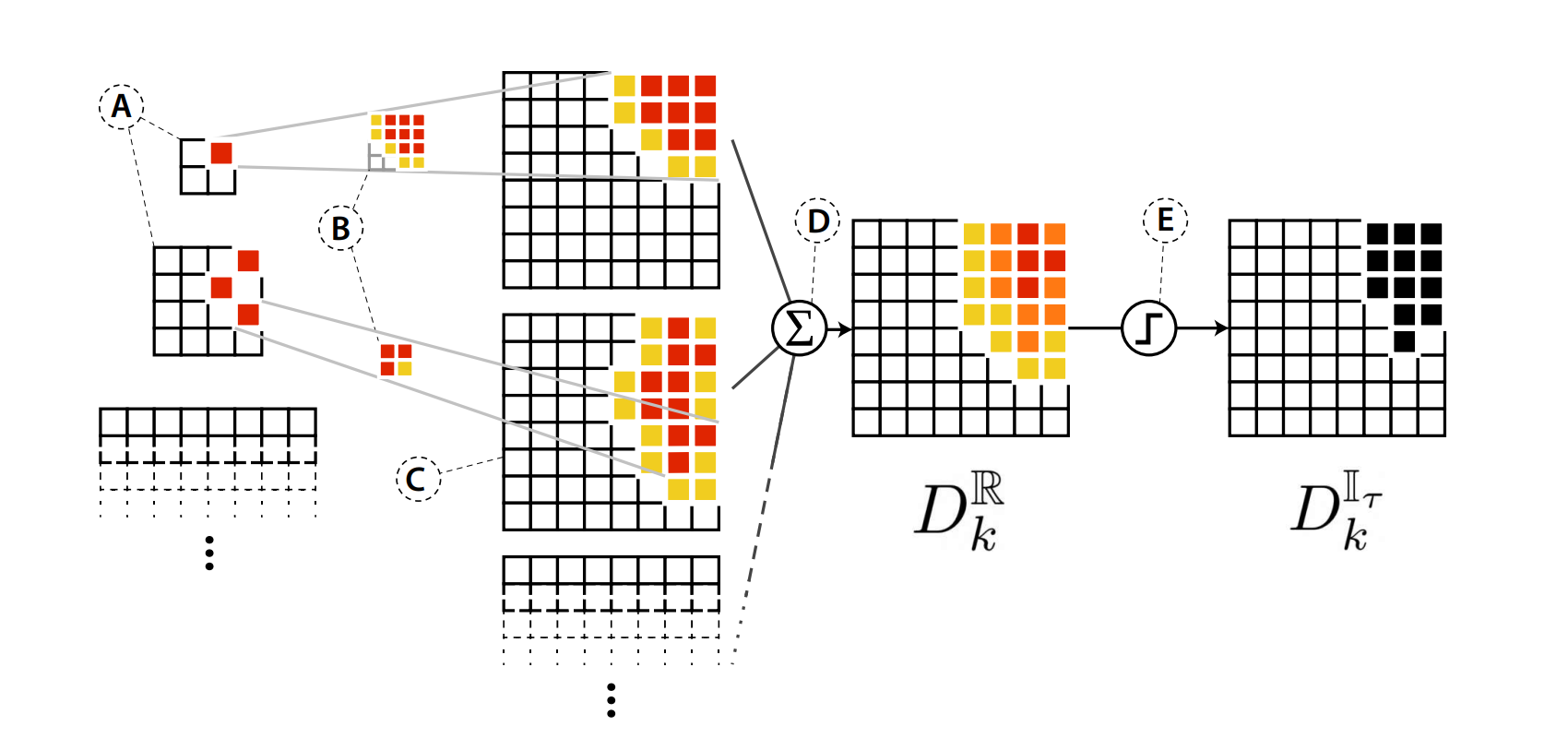
Rather than examining the aggregate differences between good and bad prompt synthesis, we next examined the difference between the conditioned and unconditioned latent at each step of diffusion. The magnitude of the difference at each position in the latent is used to create a difference map which indicates what the impact of the conditioning is on diffusion when the impact of the denoising of the model is removed. In other words, what is the impact of only the conditioning on the prompt.
Methodology
When generating an image with latent diffusion, two latents are processed in each step of size (4, 64, 64). One is conditioned on the prompt and another is unconditioned, receiving an embedded empty string as its conditioning in practice. The difference between these two latents is calculated, scaled by a factor called the guidance scale (usually around 5-10, and is a hyperparameter one can set), and then added to the unconditioned prompt. Taking the difference of these latents, we can see the model’s behavior in terms of just the prompt impact. The model denoises and conditions on the prompt at the same time in each step, but by subtracting the unconditioned latent, we can remove the exclusively denoising changes. Technically, the model predicts the noise added on each step by the noising process, which is hypothetical when running the model in inference mode to generate new images. To calculate the difference between the latent after this predicted noise has been removed for both conditioned and unconditioned noise predictions, we start with the following:
\begin{aligned} \text{new conditioned latent} &= \text{old latent} - \text{noise conditioned} \\ \text{new unconditioned latent} &= \text{old latent} - \text{noise unconditioned} \text{ }\\ \end{aligned}
\begin{aligned} \text{new conditioned latent} - \text{new unconditioned latent}\end{aligned} \begin{aligned} &= \text{(old latent} - \text{noise conditioned)} - \text{(old latent} - \text{noise unconditioned)} \end{aligned}
Which is just the difference between the predicted noise. Since we will take the L2 norm of this noise down the channel dimension, the order of subtraction does not matter.
The L2 norm of the difference between the conditioned and unconditioned latent is recorded at each step during the diffusion process. We experimented with using the other difference calculation methods explained in Probe 2, but decided against using them. Their pooling helps smooth over differences to make calculating bigger trends from the data less noisy. Here, we only look at one latent difference at a time, so this pooling is not needed. We display the difference in a map where the bigger differences appear as darker colors. This image representation of the latent appears sensicle and easily interpretable without more advanced conditioned-unconditioned difference calculations, so we chose to use the simpler difference calculation scheme.
Experiment
60 generations were performed and the latents were stored. 3 prompts were used with 20 seeds for unique images. The intermediate steps (after the scheduler removed the noise) were captured as well. The differences and intermediates after being passed through the VAE are displayed side by side or separately. There is an option in the code to display every n latent difference and intermediate as all 100 images displayed for both methods can be excessive.
Results
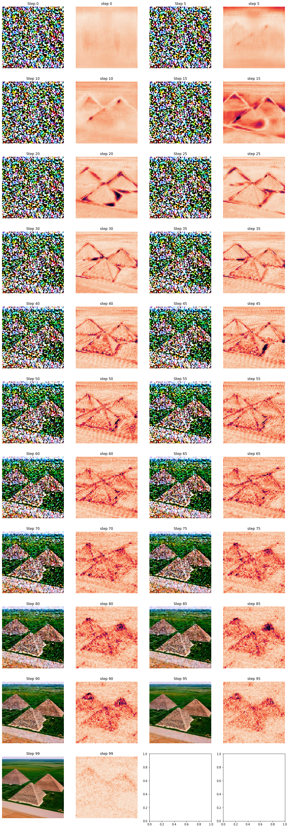
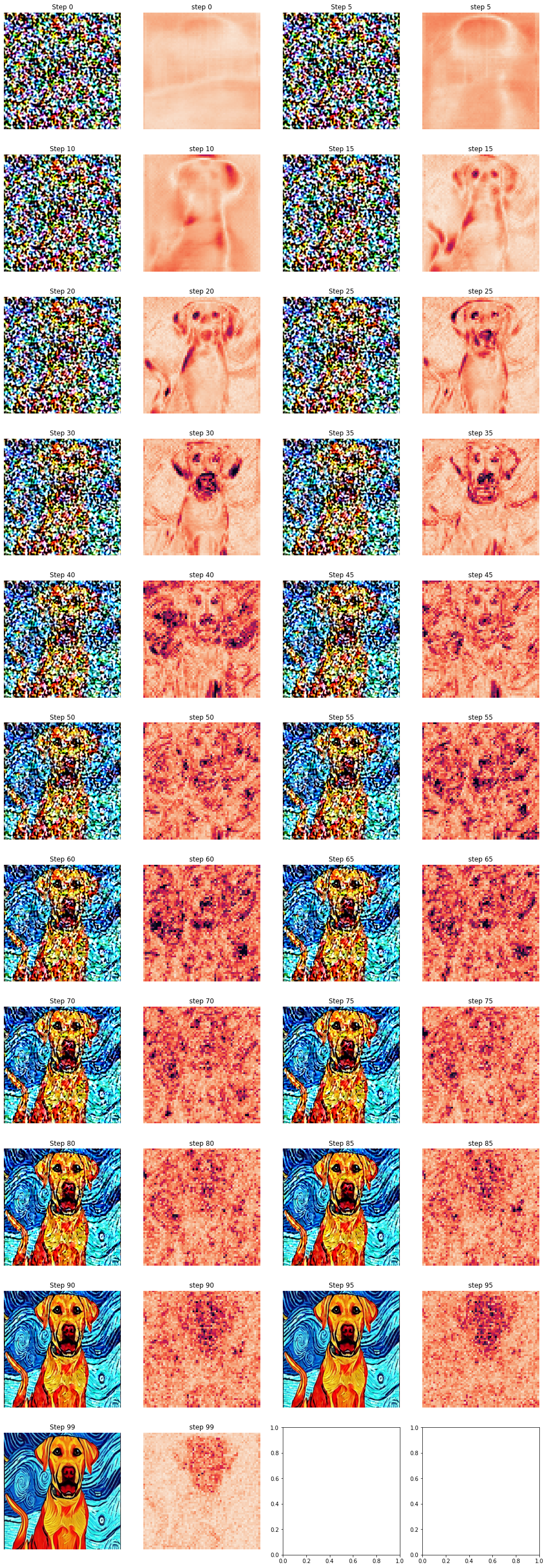
The above figure shows the traditional visualization and the difference map shown side by side. The traditional visualization shows the cumulative progress in the diffusion process while the conditioned-unconditioned difference map shows what the model is focusing on in one particular step. At step 5, we can see the conditioning already drawing the forms of the pyramid, which do not become visible in the traditional visualization until roughly 20 more steps. The model also creates a large conditioned-unconditioned difference in the area of the image that will become the sky. In step 15, the conditioned-unconditioned difference shows fields being emphasized as well as the pyramid forms. A roadway is shown with the slanted line under the pyramids. Toward the end of the diffusion, we see differences spread over the whole image. This may be texture and details being drawn. In the last 5-10 steps, the total impact of conditioning lessens as the model is mainly removing noise from a nearly complete image.
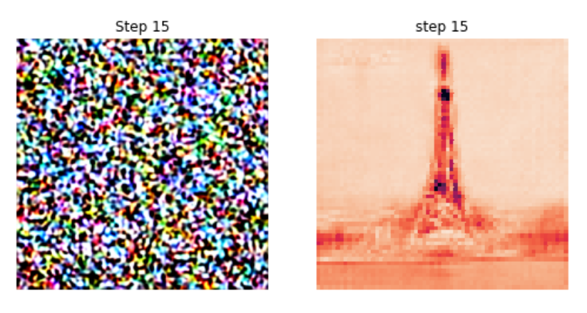
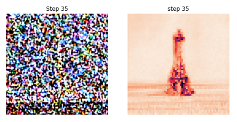
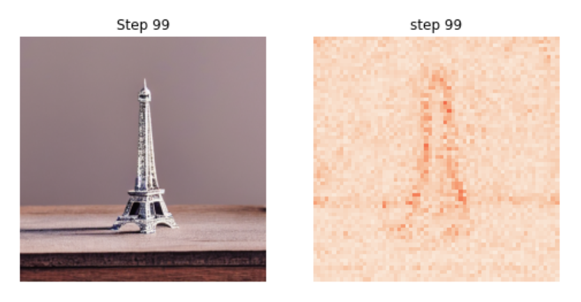
In the above figures, we again see the ideas from the prompt manifest much quicker in this new visualization compared to the traditional one. As soon as after the first diffusion step (step 0) the outline of the Eiffel Tower is visible. In step 15, details such as the deck at the top of the towner, the deck at the bottom, and the arches appear. The traditional visualization is still just uninterpretable noise. At step 25, the shadow to the left of the tower is brought about due to the conditioning. Similarly, the conditioned-unconditioned difference diminishes as the diffusion reaches the final few steps.
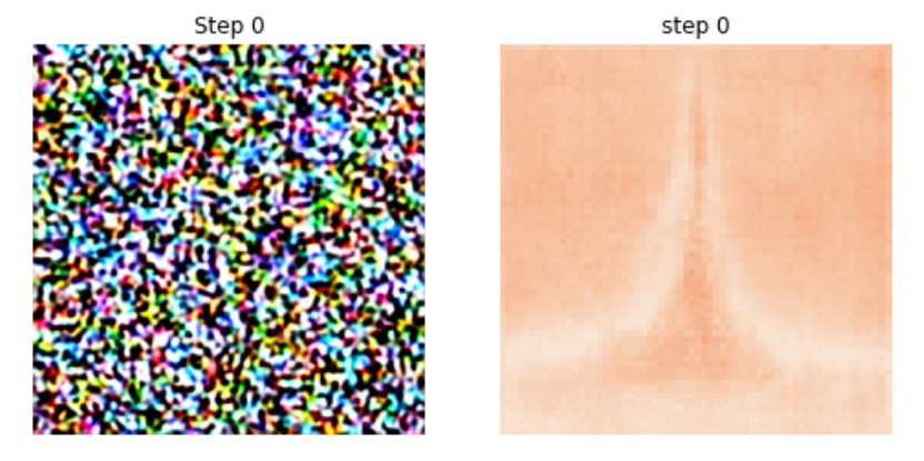
This last figure is provided to illustrate the new visualization technique once more.
Discussion
This new visualization technique pulls back the veil of the noise particularly visible in the first half of the traditional diffusion to show us what the model is working on at each diffusion step. We can see that the model rapidly starts using the conditioning to place objects from the embedded text prompt into the image. The traditional visualization does not clue us into this process as the forms of items and concepts from the text conditioning do not appear in it until much later.
This visualization allows us to see that the model does not really change its mind. After just a few steps, the outlines of the objects that appear in the final image are visible. These outlines do not change. Further, we see that the model takes an intuitive approach toward drawing. The shapes come first, then interior details. As seen in all three prompts from this section, the general form appears in about 5 steps. The details (e.g. dog’s eyes, Eiffel Tower decks) come after. The model focuses on details in the later steps, particularly the last half, This is seen in the concentration of changes. In early stages, the differences between the conditioned and unconditioned latenets are strong or not apparent–the model works on large features. In the later stages (particularly visible in the last example with the Lab) the impact of the conditioning is high across the whole image.
The inability to show color weakens this visualization. This prevents us from seeing where information from the conditioning such as “red” or “wooden” appears as these details reside in the different channels of the latent. One potential strategy to improve the visualization is to take the conditioned unconditioned difference, scale it, and add it to a latent that just produces a gray image when passed through the VAE. It is unclear how to scale the difference best for this approach or if it would work at all.
Through this new visualization, we have found trends in latent diffusion generation. The model takes a logical (from a human perspective) approach to drawing the images. The beginning steps, where it appears little progress is being made in the traditional visualization, are where major decisions about the final form are made, indicating some of the most important work of the model occurs here.
Probe 4: Probing Visual Reasoning of Stable Diffusion
Recently, models such as stable diffusion represent a significant milestone in text-Image generation, and have gained immense popularity and intrigue with the models generating hyper-realistic images for prompts such as “A photo of an astronaut riding a horse on Mars”. Such results indicate the model’s ability to compose ideas and concepts that cannot simply be picked up from some of the images in the training data distribution. However, due to the challenges in explainability and interpretability of these models, there hasn't been extensive research on the scope and limitations of these model’s visual reasoning abilities such as compositional reasoning, object recognition and counting, and spatial and object-attribute relationship understanding.
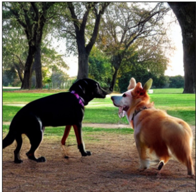
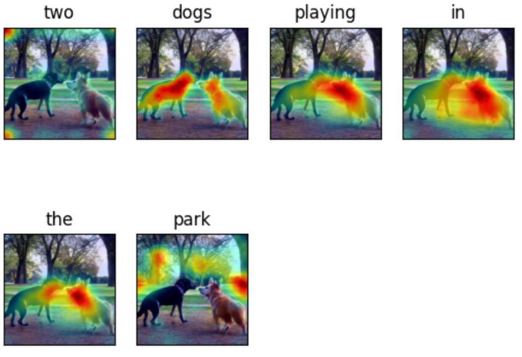
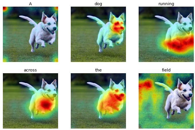
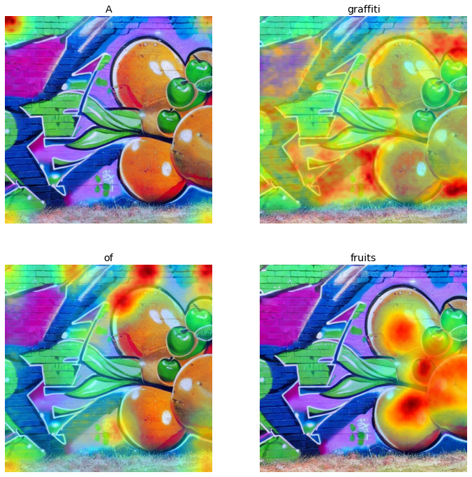
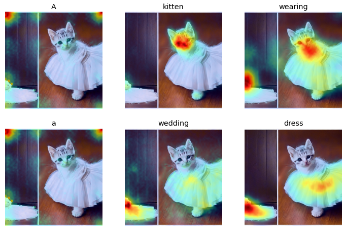
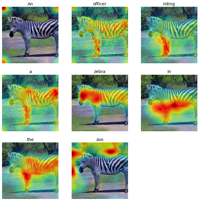
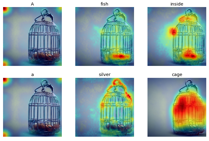
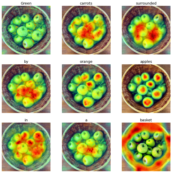
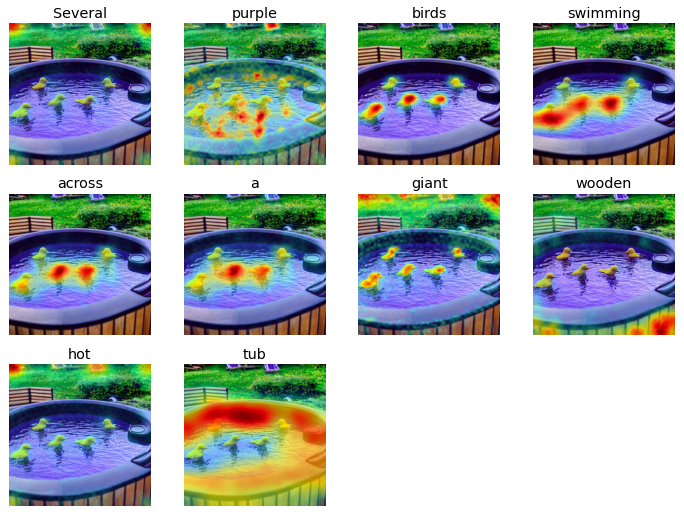
As a starting point to assess the visual reasoning abilities of the stable diffusion model, we implement the cross-attention based attribution method called DAAM to visualize the regions of most influence of each input word in a prompt on the generated image, to probe into what the model was “thinking” or paying attention to while generating the output. By assessing the patterns in attribution maps and attention distribution for different types of input words, we seek to gain a better insight into the extent of a model’s visual reasoning abilities.
Methodology
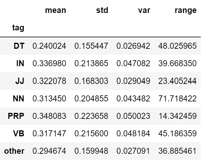
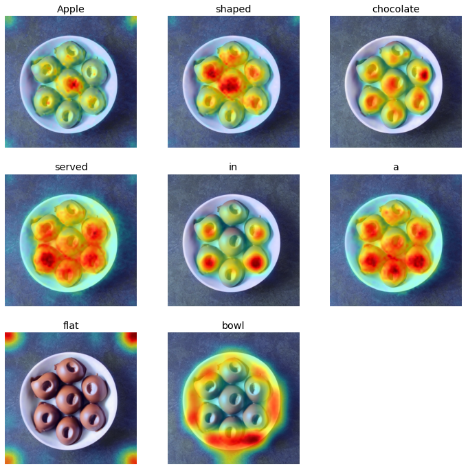
To carry out this research, we implemented the DAAM method to visualize the attention activation maps for each word of the prompt. In the initial experiment, we implemented this method to visualize the heat maps for a range of prompts that would require some compositional reasoning, action and object recognition, and counting to render realistic images. To further streamline the experiment to probe into the model’s visual reasoning abilities, the second experiment involved curating a list of 50-60 prompts sourced from the 1000 most frequently occurring words in COCO Image Caption dataset. The 1000 most frequent words were labeled with six different POS tags (NN, VB, JJ, DT, IN, PRP, and other) which also translate to different visual reasoning skills. For instance, we assume that visually, nouns (NN) and verbs (VB) correspond to object and action recognition skills, adjectives (JJ) correspond to object-attribute relationship understanding, and other categories (DT, PRP, IN, and other) correspond to spatial relation and counting understanding.
By performing a quantitative analysis of the attention weight distributions for different POS tags, we seek to compare any global patterns in the attention activations for different word types. Characterizing these patterns also helps assess the model’s performance in terms of the visual reasoning skills and identify any existing gaps in the model’s learning that could be further investigated and improved.
Experiment
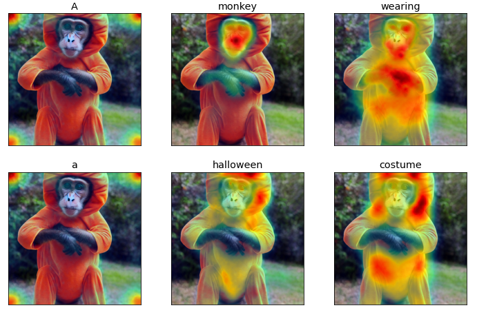
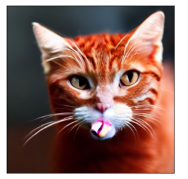
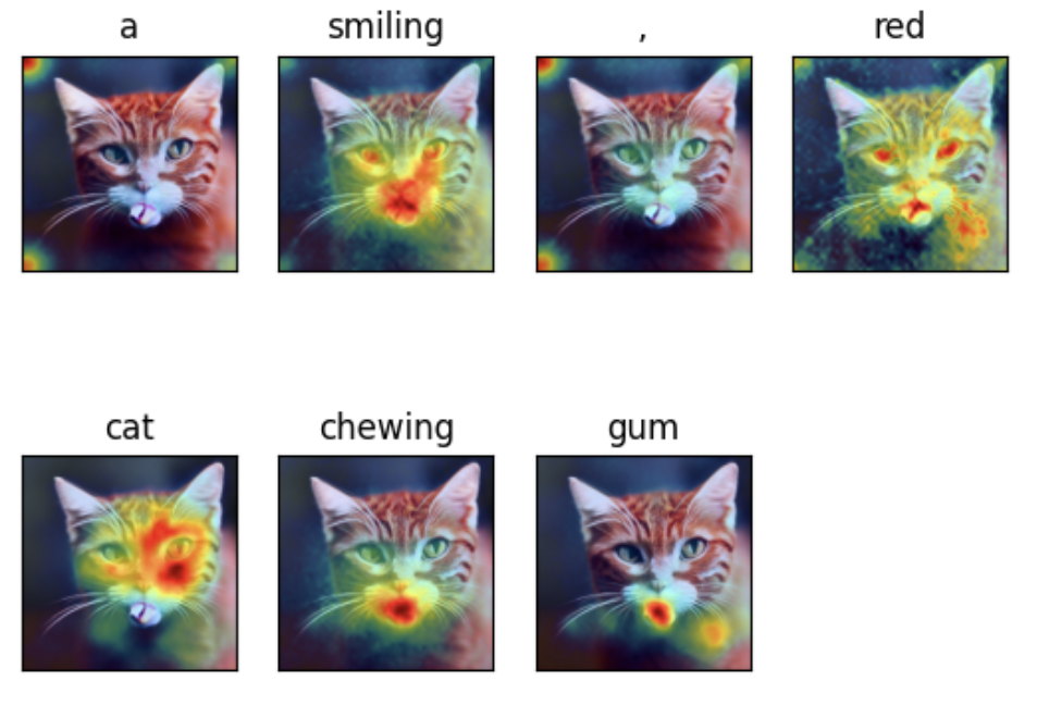
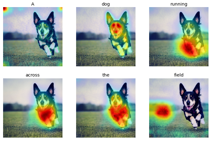
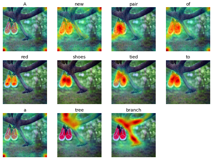
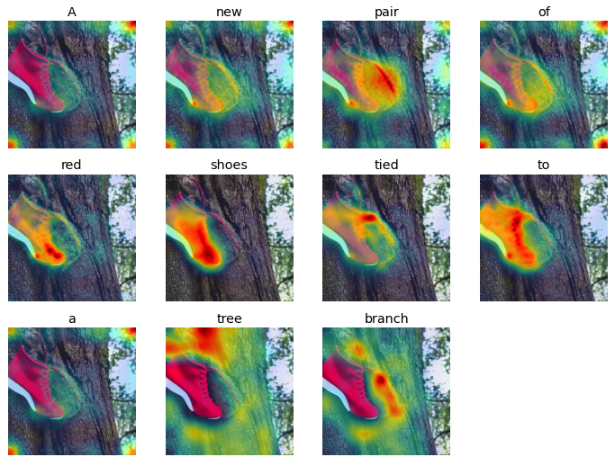
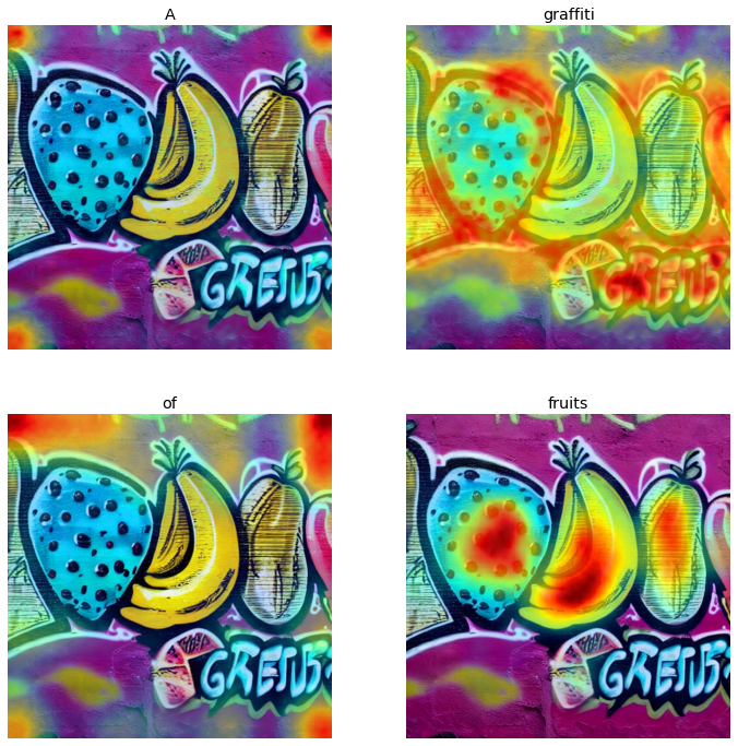
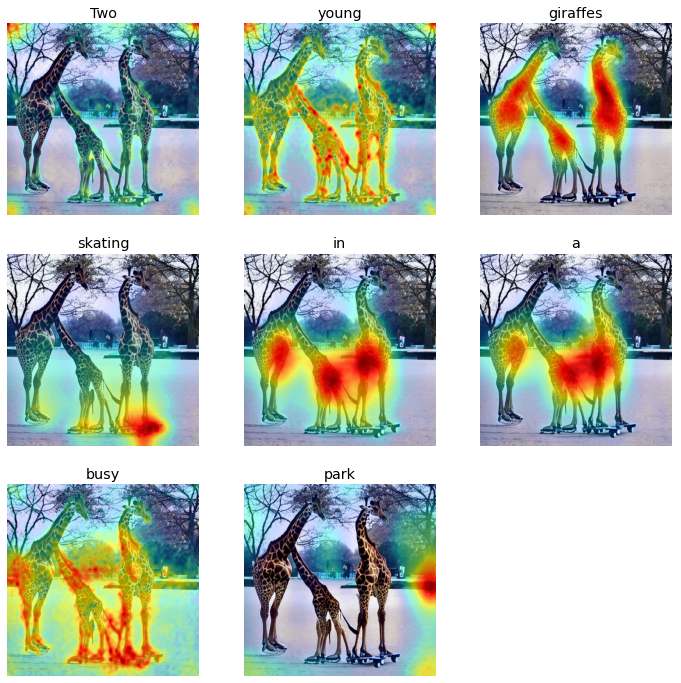
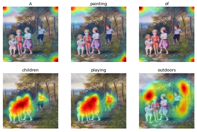
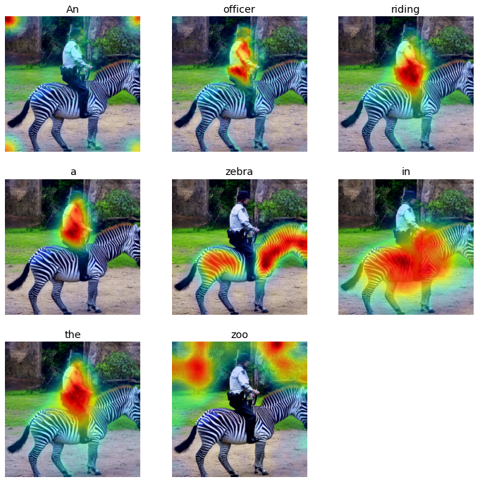
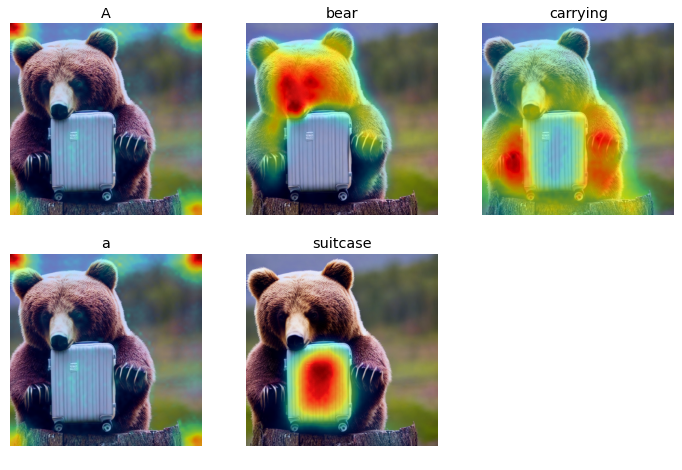
The initial analysis involved qualitatively assessing the attention activation maps for each input word using prompts that would require the model to compose different ideas and concepts to render a realistic representation. For instance, figures 2.8 represent some of the sample prompts and the resulting visualizations from the initial experiment.
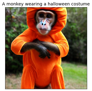
From the initial experiment, we noticed highest and accurate attention activations for nouns, and verbs, and lower activations for attributes, and words corresponding to numbers. We decided to focus more on this behavior and characterize the attention activations for common verbs, nouns, adjectives, and other words that were among the 1000 most prevalent words in the COCO image caption dataset. We chose this dataset as this data was used to train the stable diffusion model and could help streamline the experiment by designing prompts using words more familiar to the model. This dataset was tagged with six categories of POS tags to help compare attention weights distribution across different word types.
Using this approach, the second experiment involved visualizing the attention maps for 50-60 different prompts designed to test different visual reasoning abilities of the model. The results from these experiments are summarized below.
Results
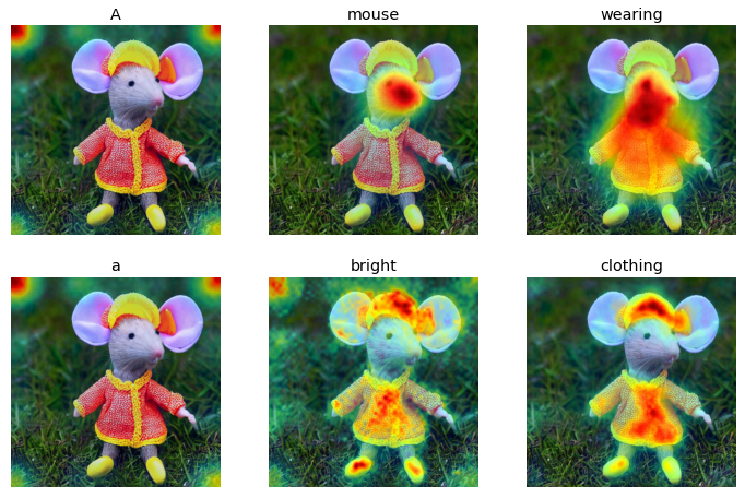
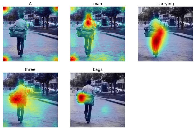
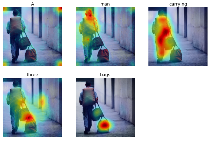
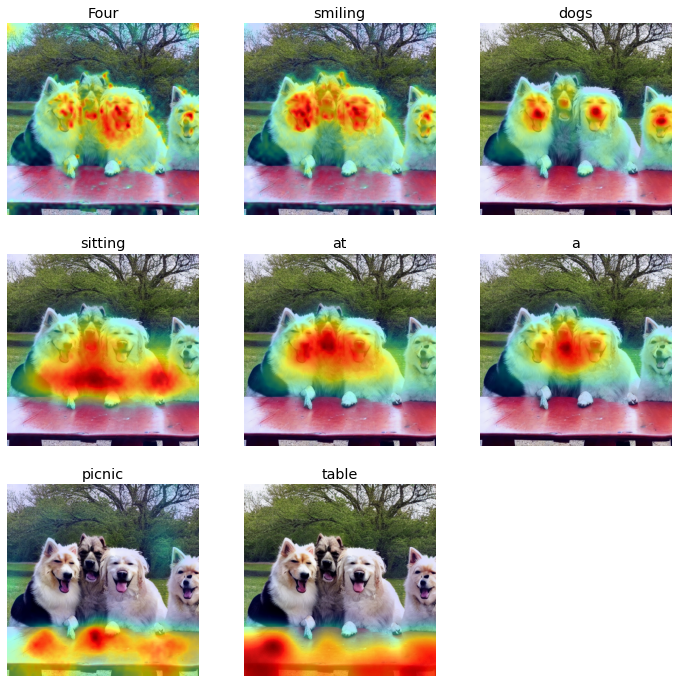
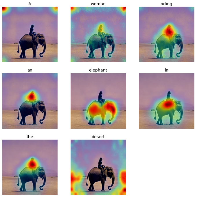
From the initial experiments, there were some distinct characteristics between the attention heat maps for input words corresponding to nouns and verbs versus those representing numbers, and determiners. While the nouns and verbs showed highest activations around regions representing the input words, the adjectives, numerals, and other word types mostly showed lower and more spread out attention activations. This could be attributed to the fact that adjectives, numerals, and other word types represent more generic concepts than verbs and nouns, which might be easier to recognize for the model.
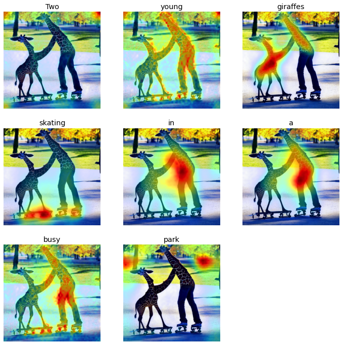
In the additional experiments, after carrying out several experiments using the “Comp Vis V1.4” and “Runway ML” stability diffusion models for 30 and 60 inference steps on 50-60 prompts curated from the frequent words from COCO caption dataset, we found similar behavior from the models overall. Some of the visualization results for different categories of prompts are shown in the tables 2.2 and 2.3 below.
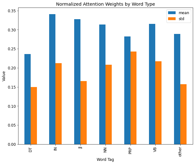
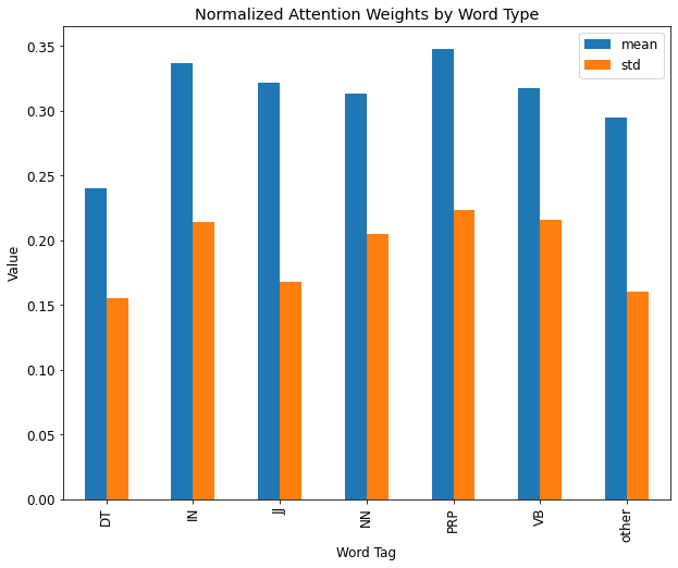
In addition to the visual qualitative experiment, we computed the mean and standard deviation of the normalized attention scores for each input word across 50-60 prompts and categorized them by their POS tags, and plotted the corresponding plots for each category. These plots are shown in Figure 2.9
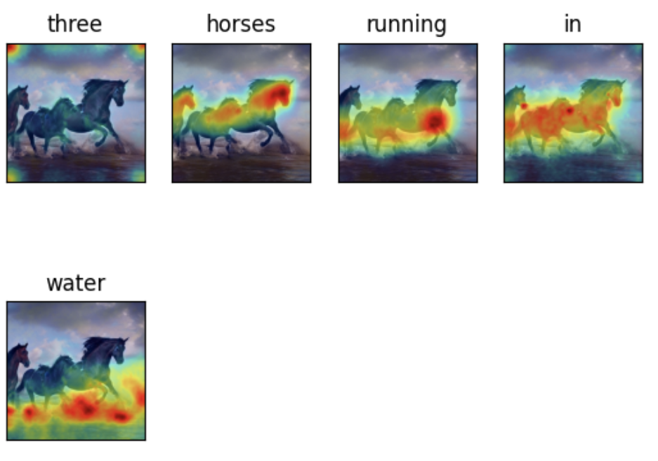
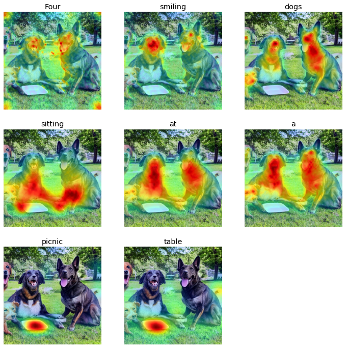
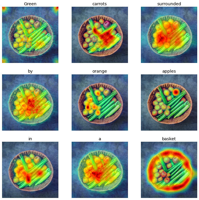
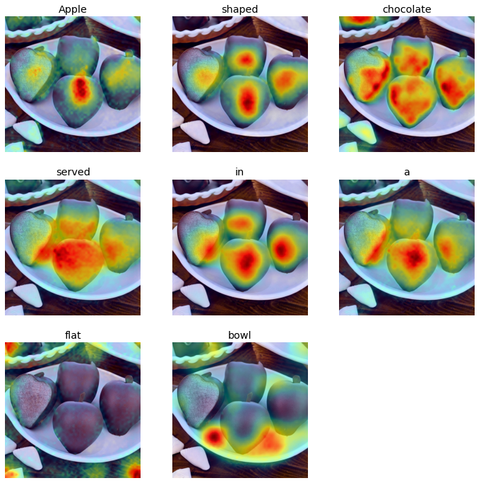
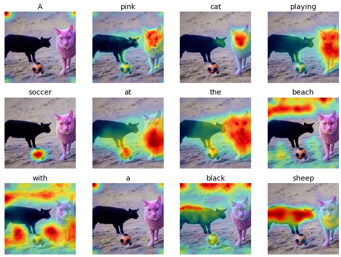
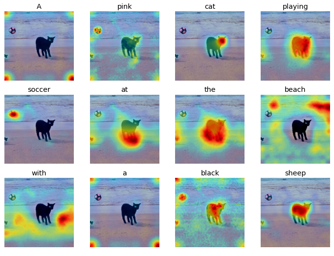
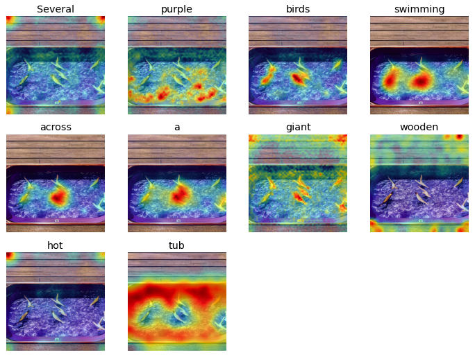
Upon testing different visual skills of the two versions of the stable diffusion model, a similar pattern from the initial experiment was observed in the attention distribution characteristics. For the nouns and verbs based input words, the models generally displayed a strong and accurate attention map aligning with the actions and objects represented by the prompt, thus indicating a relatively more accurate object and action recognition skills. However, the attention weights’ patterns for numerals and other word types representing spatial and multiple object-attribute relationship understanding showed a weaker and lower alignment between words and heat map patterns.
|
Skill: Object & Action Recognition
(Generating specific objects doing specific actions)
|
Skill: Object Counting
(Generating specific number of objects)
|
||||
|---|---|---|---|---|---|
|
Model
|
Runway ML Stable Diffusion V1.5
|
Com Vis Stable Diffusion V1.4
|
Runway ML Stable Diffusion V1.5
|
Com Vis Stable Diffusion V1.4
|
|
|
Prompt: A dog running across the field
|
Prompt: A new pair of red shoes tied to a tree branch
| ||||
|
|
|
|
||
|
Prompt: A graffiti of fruits
|
Prompt: Two young giraffes skating in a busy park
|
||||
|
|
|
|
||
|
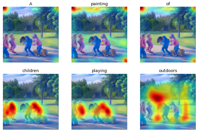
Prompt: A painting of children playing outdoors
|
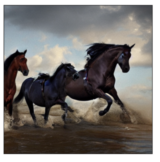
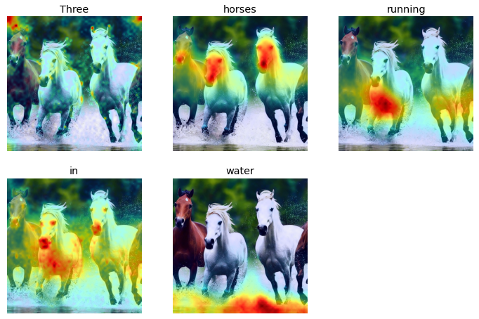
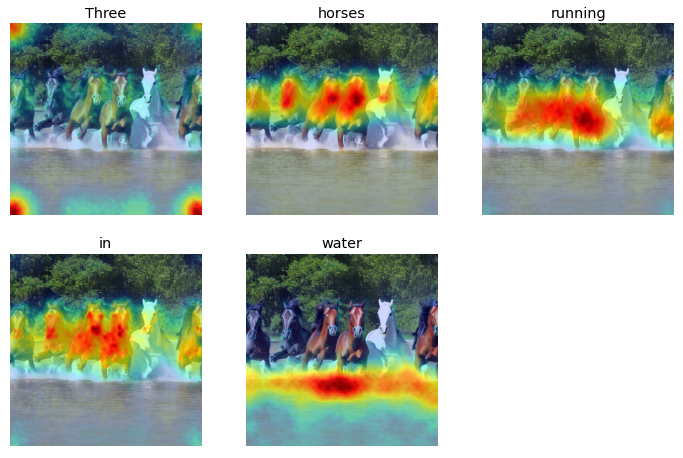
Prompt: Three horses running in water
|
||||
|
|
|
|
||
|
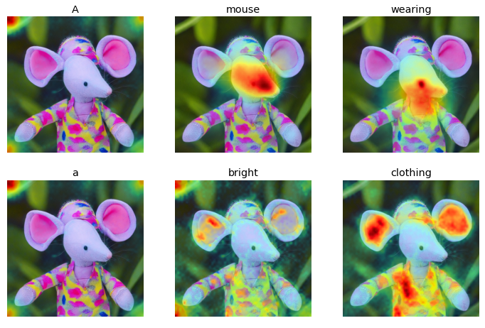
Prompt: A mouse wearing a bright clothing
|
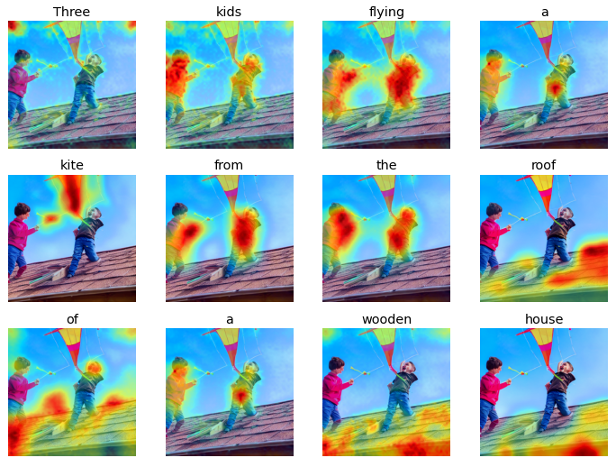
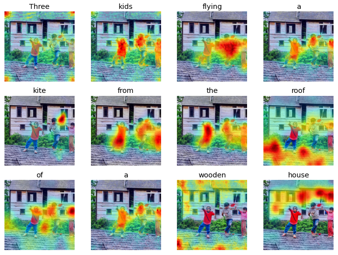
Prompt: Three kids flying a kite from the roof of a wooden house
|
||||
|
|
|
|
||
|
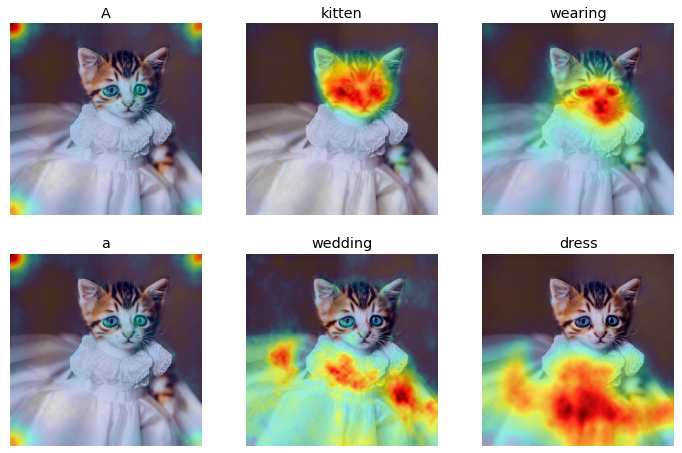
Prompt: A kitten wearing a wedding dress
|
Prompt:A man carrying three bags
|
||||
|
|
|
|
||
|
Prompt: An officer riding a zebra in the zoo
|
Four smiling dogs sitting at a picnic table
|
||||
|
|
|
|
||
|
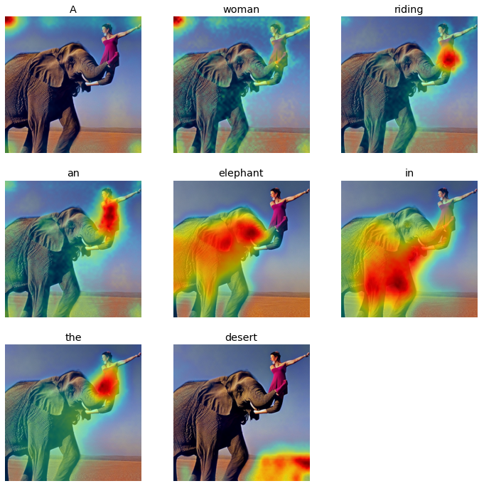
Prompt: A woman riding an elephant in the desert
|
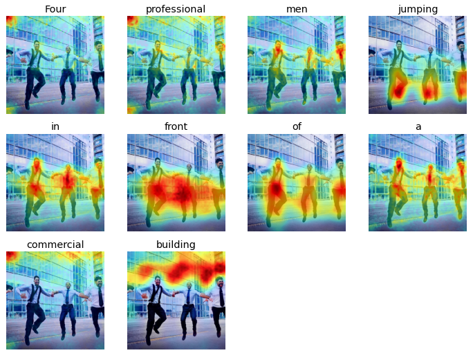
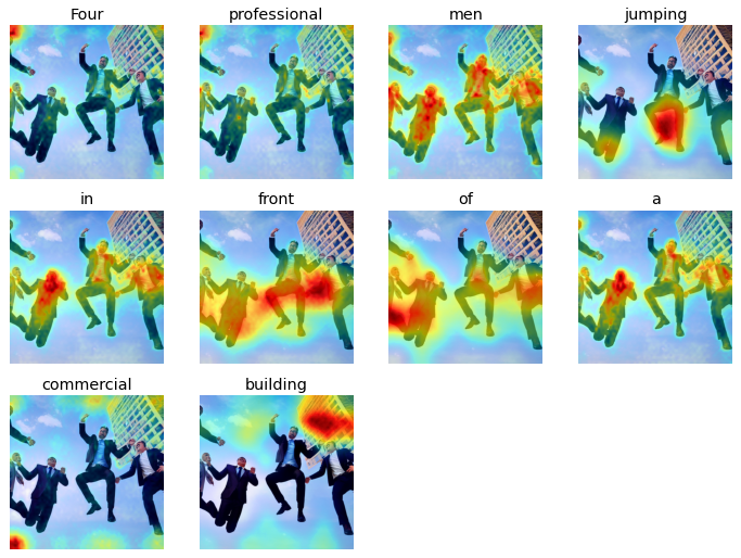
Prompt: Four professional men jumping in front of a commercial building
|
||||
|
|
|
|
||
|
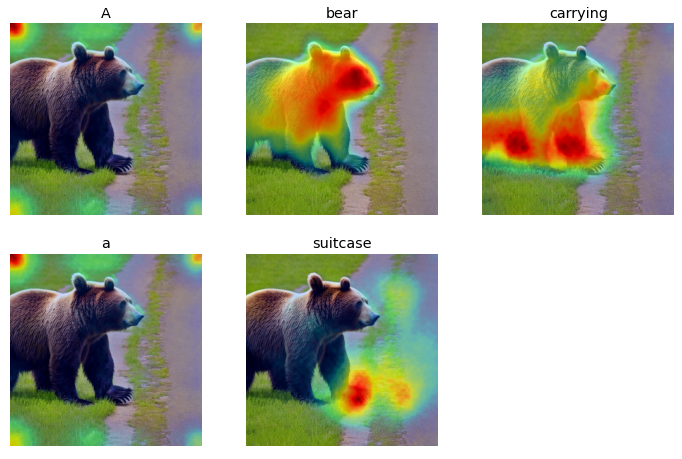
Prompt: A bear carrying a suitcase
|
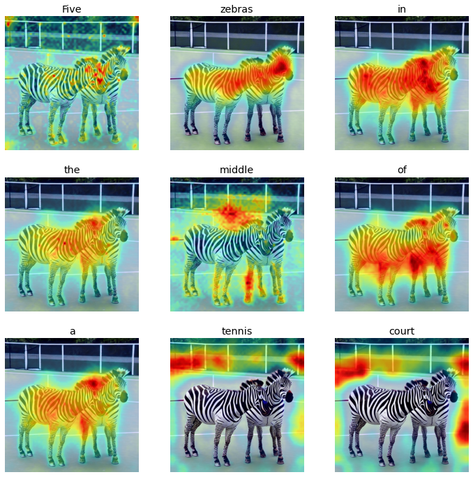
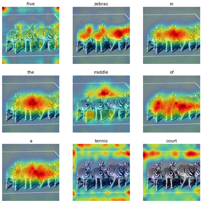
Prompt: Five zebras in the middle of a tennis court
|
||||
|
|
|
|
||
|
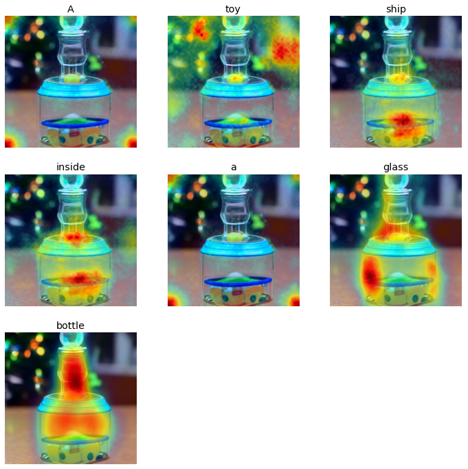
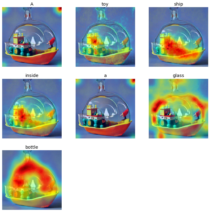
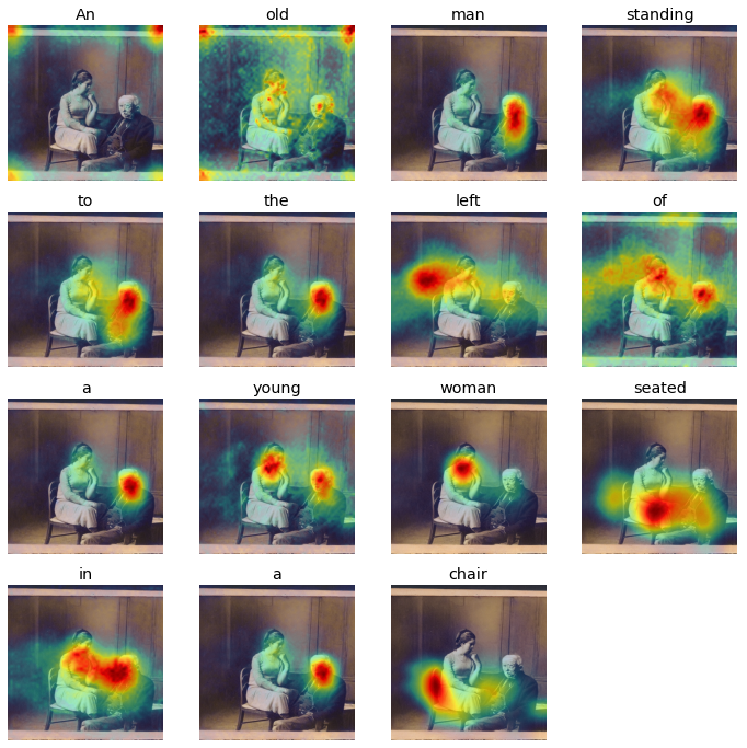
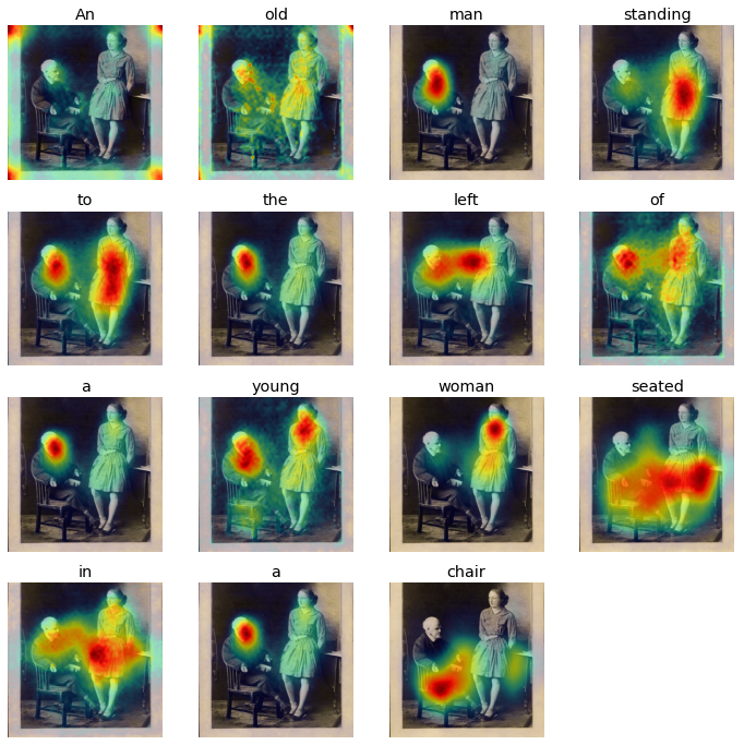
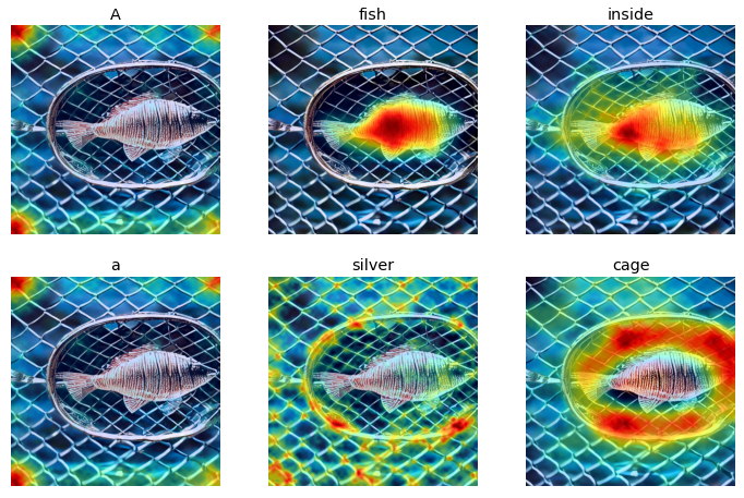
Skill: Spatial and Object-Attribute Relationship
(Generating specific objects with different spatial relation or attributes)
|
||
|---|---|---|
|
Model
|
Runway ML Stable Diffusion V1.5
|
Com Vis Stable Diffusion V1.4
|
|
Prompt: A toy ship inside a glass bottle
|
||
|
|
|
|
Prompt: An old man standing to the left of a young woman
|
||
|
|
|
|
Prompt: A fish inside a silver cage
|
||
|
|
|
|
Prompt: Green carrots surrounded by orange apples in a basket
|
||
|
|
|
|
Prompt: Apple shaped chocolate served in a flat bowl
|
||
|
|
|
|
Prompt: A pink cat playing soccer at the beach with a black sheep
|
||
|
|
|
|
Prompt: Several purple birds swimming across a giant wooden hot tub
|
||
|
|
|
|
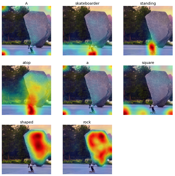
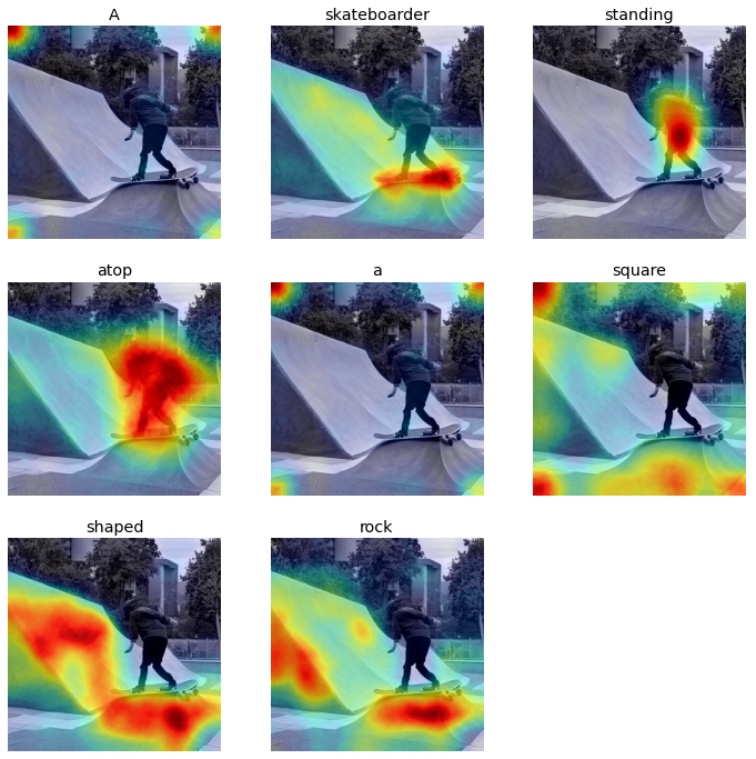
Prompt: A skateboarder standing atop a square shaped rock
|
||
|
|
|
|
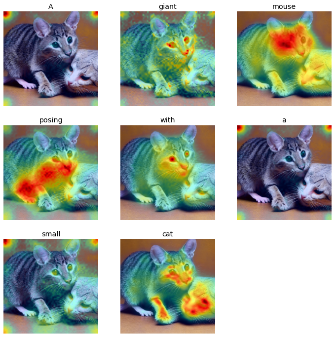
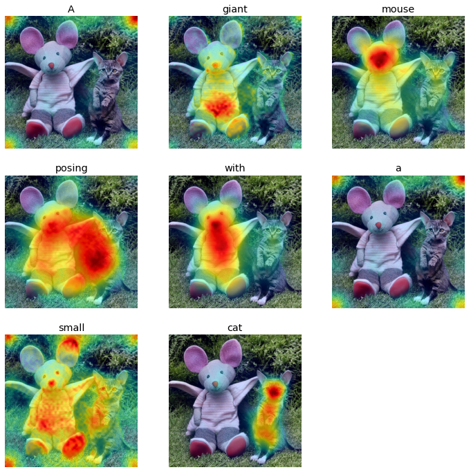
Prompt: A giant mouse posing with a small cat
|
||
|
|
|
Limitations
In our experiments, we have worked with a limited set of prompts and attempted to do some quantitative evaluations in addition to qualitative analyses. However, additional experiments would be needed to validate and understand the patterns we have observed in these experiments. In addition, for probe 4, we used the 1000 most frequent words from the COCO caption dataset, which consisted of an unequal distribution of POS tags, which might have limited our ability to assess the attention weights distribution patterns more accurately. So, the future experiments could investigate a uniform number of words from different tags for examining more generalized patterns in the attention weights.
Conclusion
Overall, through our multiple experiments in our research, we have probed and evaluated the diffusion model’s behavior and the diffusion process, and explored the extent and limitations of its visual reasoning abilities. In addition, we have also explored the extent of visual and compositional reasoning capability of the model and characterized the qualitative and quantitative patterns we have observed through our experiments. To discover more about the diffusion process, we constructed four probes that reveal behavior of the model not observable in the traditional visualization.
In probe 1, we observed a general trend in the diffusion process by altering the scheduling mid run to a schedule that informs the model to quickly finish the diffusion. Through this experiment, we observed that the model is performing useful actions that move it towards a clean coherent image earlier than one would assume when using the traditional visualization. The interesting effect where the quick finish degrades quality in later runs motivated us to seek alternate visualizations or metrics that inform us of the model’s actions and progress throughout the diffusion process.
In Probe 2, we examined the magnitude of the difference between the conditioned and unconditioned prompts. Through probe 2, we observed that the model may not use the prompt when altering the fine details of the image, which matches with the traditional visualizations’ insights, where the image loses some unnatural color and brightness noise, and appears independent of the actual content. Through probe 3, we visualized the conditioned-unconditioned difference map to see what the model is focusing on in one particular step. Overall, both Probes 1 and 3 both indicated that the model takes only a few steps to determine the sketch of the final output and showed the model’s focus at various steps.
Apart from exploring the diffusion process, in Probe 4, we implemented the diffusion attentive attribution maps (DAAM) method to visualize the stable diffusion model’s regions of influence for each input word in the prompt and quantify the attention weights distribution. Both quantitative and qualitative analyses indicated that the model has a higher understanding of actions and objects based on the prompts compared to their counts and relationships.
In addition, in some cases, we observed a varied performance of the model with accurate representations of all the components of the prompts in some cases, and missing objects or misalignment of spatial and object-attribute relationships in the other.
Citations
- Ho, J., Jain, A., & Abbeel, P.. (2020). Denoising Diffusion Probabilistic Models.
- Rogge, N.,& Rasul, K.. (2022). The Annotated Diffusion Model
- Rombach, R., Blattmann, A., Lorenz, D., Esser, P., & Ommer, B. (2022). High-Resolution Image Synthesis With Latent Diffusion Models. In Proceedings of the IEEE/CVF Conference on Computer Vision and Pattern Recognition (CVPR) (pp. 10684-10695).
- Sergey Zagoruyko and Nikos Komodakis. Wide residual networks. arXiv preprint arXiv:1605.07146, 2016.
- Blog post titled “Stable Diffusion with 🧨 Diffusers” published 22 August 2022 by Suraj Patil, Pedro Cuenca, Nathan Lambert, and Patrick von Platen.
- Tang, R., Pandey, A., Jiang, Z., Yang, G., Kumar, K., Lin, J., & Ture, F. (2022). What the DAAM: Interpreting Stable Diffusion Using Cross Attention. arXiv preprint arXiv:2210.04885.
- Fong, R., Patrick, M., & Vedaldi, A. (2019). Understanding deep networks via extremal perturbations and smooth masks. In Proceedings of the IEEE/CVF international conference on computer vision (pp. 2950-2958).
- Alvarez-Melis, D., & Jaakkola, T. S. (2018). On the robustness of interpretability methods. arXiv preprint arXiv:1806.08049.
- Zeiler, M. D., & Fergus, R. (2014, September). Visualizing and understanding convolutional networks. In European conference on computer vision (pp. 818-833). Springer, Cham.
- Chen, X., Fang, H., Lin, T. Y., Vedantam, R., Gupta, S., Dollár, P., & Zitnick, C. L. (2015). Microsoft coco captions: Data collection and evaluation server. arXiv preprint arXiv:1504.00325.
- Cho, J., Zala, A., & Bansal, M. (2022). Dall-eval: Probing the reasoning skills and social biases of text-to-image generative transformers. arXiv preprint arXiv:2202.04053.
- Blog post titled “The Illustrated Stable Diffusion” published November 2022 by Jay Alamar.
Appendices
Code Links
-
Diffusion Model: Notebook where the diffusion model is run for Probes 1-3. This notebook generates images with latent diffusion and stores the results. Intermediates and other metrics are recorded as well. -
Quick finish: Notebook where the Quick Finish Strategy is explored. -
Conditioned-unconditioned differences per prompt. Notebook where the conditioned-unconditioned differences are analyzed from Probe 2. This analysis is for each prompt separately. -
Aggregate conditioned-unconditioned differences. Notebook where the aggregate conditioned-unconditioned differences are analyzed from Probe 2. Here, the results from the 130 runs are examined as a whole. -
Conditioned-unconditioned difference map visualization. Notebook where the conditioned-unconditioned difference’s nature is examined. This notebook corresponds with Probe 3. -
Latent diffusion pre-computed. Data folder holding the outputs and intermediate variables for many diffusion runs. Many notebooks pull from the folder. It is easier to generate many images and then pull from the stored results rather than load and run the diffusion model on demand as the model required GPU and high amounts of RAM. -
Results for aggregation. Data Folder holding the results from aggregating the conditioned unconditioned differences. This folder is needed for the notebook “Aggregate conditioned-unconditioned differences”